Attributes in Q-SoPrA

Introduction

One of the tasks that you are likely to use Q-SoPrA for is the qualification of incident data, by assigning codes to them (see this earlier post for an explanation of what incidents are). The tools you will use for this are not very different from those that you would typically use to assign codes to interviews or the contents of documents when using CAQDAS software. In Q-SoPrA, the codes that are used to qualify incident data are referred to as attributes.

You can use attributes to capture any information included in incident data that is meaningful for your study. For example, you could use attributes to distinguish between different types of activities, to identify actors or other entities involved in incidents, to record changes in variables associated with the incidents, and so on. What exactly you will use attributes for will depend heavily on your research question(s), and the theoretical basis of your research. You might of course also use attributes in a ‘grounded research’ approach, where you develop attributes on the fly, and develop these further as you proceed with your project. In this post I try to be mostly agnostic to different ways in which attributes might be used, while discussing various ways in which attributes (can) play a role when using Q-SoPrA in research projects.

In this post I discuss four main topics. I first discuss some basic, somewhat technical details of what attributes in Q-SoPrA are, how they can be organised, and how they are stored, and so on (but this is really quite simple). I then discuss different ways in which attributes can be assigned to incidents (and more abstract events; more on this later). This is followed by a brief discussion of various other simple ways to interact with attributes. Finally, I discuss some ways in which attributes can be used in visualisation and analysis.

Attributes in Q-SoPrA

Attributes have to be defined by the user. There are three different widgets in which this can be done, but the most obvious ‘place’ to define new attributes is the Attributes Widget (see screenshot below).

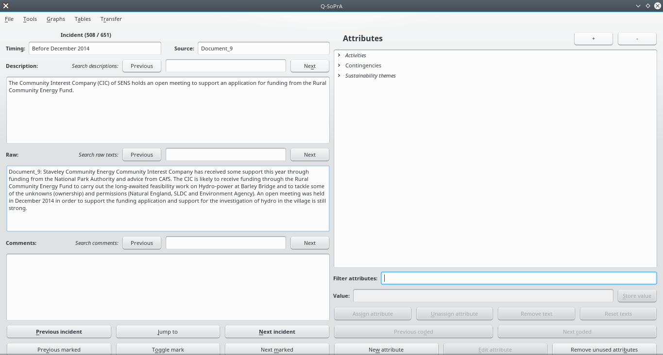
On the left side of this screen you see some fields that show the data associated with the incident that is currently being inspected (the timing, source, description, raw source text, and other comments/memos written by the analyst). On the right side of the screen you can see the attributes view. When you create a new database, this view will be empty. In the bottom-right of the screen you see all controls that are specifically associated with attributes. For example, you find controls to define new attributes, to edit existing ones, to assign the currently selected attribute to the present incident, and etcetera.

Creating new attributes

We will focus first on the creation of new attributes. Attributes in Q-SoPrA can be understood to have three main properties:

1. All attributes have a unique label (or name);
2. All attributes have a description (or definition);
3. Attributes can have a parent attribute.

To create a new attribute, click the New Attribute button. This will open the dialog shown below.

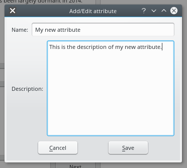
You are always required to provide a label and a description for your attributes. If one of these is missing, then Q-SoPrA won’t allow you to save the attribute. Also, the name of the attribute has to be unique. The idea behind forcing you to provide a description is to make you think immediately about the definition of your attribute, and about the phenomena that your attribute is supposed to capture.

Attribute hierarchies

I mentioned above that attributes can have parents. That is, attributes in Q-SoPrA can be hierarchically organised by assigning parents/children to them. A parent is automatically assigned to a new attribute if you select an existing one before clicking the New Attribute button. In this case, the new attribute will be created as a child of the existing attribute you selected. You can re-parent attributes by dragging and dropping them onto other attributes. If you drag an attribute to an empty space in the attribute view, the attribute will be ‘orphaned’, and appear in the highest level of the attribute hierarchy. In this way, you can create as many hierarchical levels of attributes as you like.

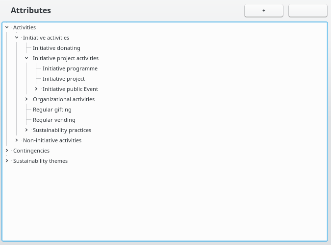
The position of an attribute in the hierarchy has important consequences. An attribute that has a parent is always considered as a sub-type of that parent. For example, if you have an attribute called Activities, and you have another attribute called Night-time activities that is a child of Activities, then Q-SoPrA assumes that Night-time activities are a kind of Activities. In this way, any attribute can serve as a sort of category for other attributes.

The specific organisation of your attributes hierarchy will be important in, among other things, the identification of ‘modes’ in your event graph (modes are discussed in a bit more detail further below): When you create a new mode based on the attribute Activities, then all incidents and events that were assigned an attribute that is a child of Activities (or grandchild, or great-grandchild, or great-great… Well, you get the idea) will also be considered to belong to that mode.

Like all other data imported into, or created with Q-SoPrA, attributes are stored in sql tables. One of these tables simply lists the names, descriptions and parents of attributes. The parent of an attribute is either (1) one of the other attributes, or (2) a string called 'NONE', which tells Q-SoPrA that the attribute exist at the highest level of the attributes hierarchy.

Assigning attributes

After you create an attribute, you can assign the attribute to incidents in your data set. The attributes widget lets you scroll through all incidents in your data set, and assign attributes to them. Assigning an attribute to an incident can be done by first selecting it in your attributes tree, and then clicking the Assign attribute button.

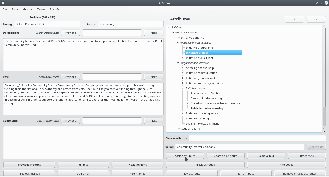
If an attribute has been assigned to the incident that you are currently inspecting, it will show up in the attributes tree with a bold font. If an attribute has a child that has been assigned to the currently inspected incident, then it will show up in the attributes tree with an italic font. If an attribute is assigned to the incident, and also has a child that was assigned to the same incident, it will show up with a font that is both italic and bold.

After assigning an attribute, it is also possible to give the attribute a value. This value can be anything from a numeric value to a string of words. Assigning a value can only be done after assigning the attribute itself. The value can be typed into the appropriate field (the Value field below the attributes tree), and then stored by clicking the Store value button (which is greyed out in the screenshot above).

Combinations of attributes and incidents are stored in a separate sql-table. Each row in this table records (1) the name of the attribute, (2) the ID of the incident that the attribute was assigned to, and (3) the value of the attribute (if one was assigned).

You may have noticed in the screenshot above that a small fragment of the text in the Raw field is highlighted (it is underlined and it is bolded). As I explained in a previous post, the Raw field is used to record any fragments of text from your sources (for example, interviews, documents, news items, and etcetera) that were the basis for creating the incident. Q-SoPrA allows you to associate fragments of text in the Raw field with attributes that you assign to incidents (you can also assign an attribute without highlighting text). Associating a fragment of text with an attribute can be achieved by (1) selecting the attribute, (2) selecting a piece of text with your mouse cursor, and (3) then clicking the Assign attribute button. Even when an attribute has already been assigned, you can assign additional fragments of text to the attribute by using this procedure. If fragments of text are assigned to an attribute, these will be highlighted whenever the attribute is selected.

The fragments of text assigned to combinations of attributes and incidents are stored in yet another sql table. In this case the rows of the table record (1) the name of the attribute, (2) the name of the incident that the attribute was assigned to, and (3) the fragment of text that is associated with the attribute-incident combination. Multiple fragments of text may exist per attribute-incident combination.

Assigning attributes in the Event Graph Widget

There are two other ‘places’ in Q-SoPrA where attributes can be assigned to incidents (or events). One of these places is the Event Graph Widget. I won’t go into the details of the Event Graph Widget here, but, briefly, the Event Graph Widget is what you will use to visualise (1) incidents and/or events, and (2) relationships between these incidents/events. An event graph gives an abstract overview of the process of interest, and how different developments in the process are related.

You can also use the Event Graph Widget to build more abstract events from your incident data. I will dedicate a future post to an explanation of how exactly this works, but the basic idea underlying the creation of abstract events is that you take a group of inter-related incidents, and say that these together constitute some larger event. For example, we might have a few incidents that capture meetings between actors ‘X’ and ‘Y’ that took place over time, and group these together in an event that we describe as ‘X and Y meet over an extended period of time.’ Abstract events are different from your incidents, because they are constituted from incidents, and thus an additional level above your data (or even more than one level, because you can also use abstract events as building blocks for yet more abstract events).

In the screenshot below you see an example of an event graph that includes incidents, as well as an abstract event that has been built from incidents.

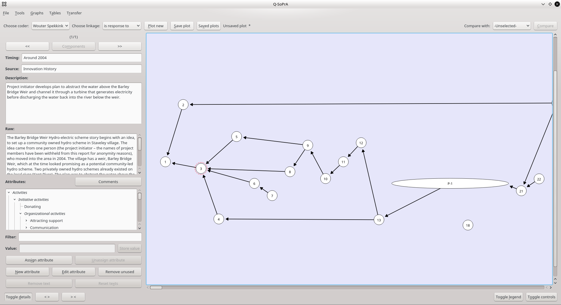
In the screenshot above, notice how the labels of most nodes are numbers, whereas there is one node (the wide elipse) that has the label "P-3". This node is an abstract event, and the labels of abstract events are based on what type of constraints were used when creating them. I will discuss the details of the possible constraints in a future post.

If you are curious, check out Peter Abell's approach to abstracting narrative graphs, as outlined in his book "The Syntax of Social Life" (1987), which is unfortunately very hard to get hold of for a reasonable price (I got lucky one time). I based two types of constraints on Abell's approach: (1) path based constraints (which are quite severe) and (2) semi-path based constraints (which are far less severe). The label of an abstract event will always start with a "P-" if it was created with path based constraints, and it will always start with an "S-" if it was created with semi-path based constraints.

In the left part of the screenshot, you see some details of the currently selected incident (the same details you would see in the Attributes Widget), as well as an attributes tree. In the Event Graph Widget, you can select any incident, and then assign attributes to them in the same way you would do this in the Attributes Widget.

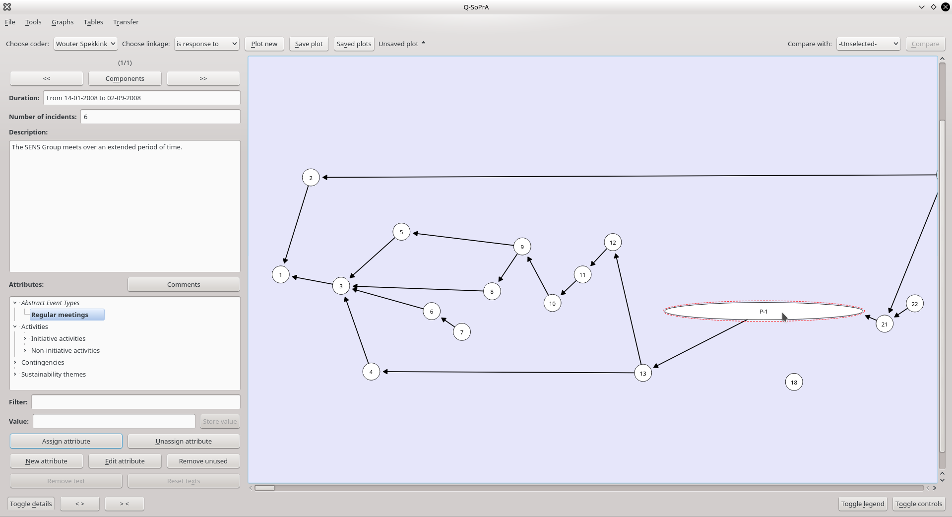
One important difference is that, in this case, you can also assign attributes to abstract events. This works largely in the same way (you select an abstract event in the event graph, after which you can assign attributes), with the exception that you cannot associate a particular fragment of text with the attribute-event combination. This is because the abstract events don’t have ‘raw’ data directly associated with them (indeed, ‘raw’ data can still be indirectly associated, through the incidents that constitute abstract events). Abstract events therefore don’t have a Raw field (see the screenshot below).

Assigning attributes in Hierarchy Graphs

Say that you have created an event graph in which you have abstracted numerous events. In the event graph, the incidents and events that were made into components of more abstract events are no longer visible themselves. This is a problem when you want to inspect those incidents and events, or when you want to change something in the attributes that you assigned to them. This is why I introduced Hierarchy Graphs to Q-SoPrA. Hierarchy graphs visualise the complete hierarchy of a given abstract event in your visible event graph. A hierarchy graph for a given abstract event can be inspected by selecting the event in your event graph, and then clicking the Components button (see screenshot below);

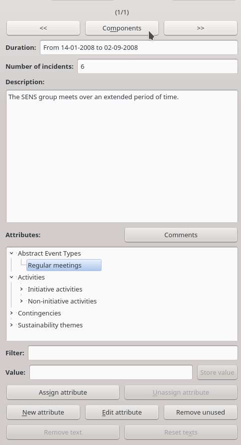
Clicking this button will cause Q-SoPrA to switch to the Hierarchy Graph widget, where the hierarchy of the currently selected event will be visualised.

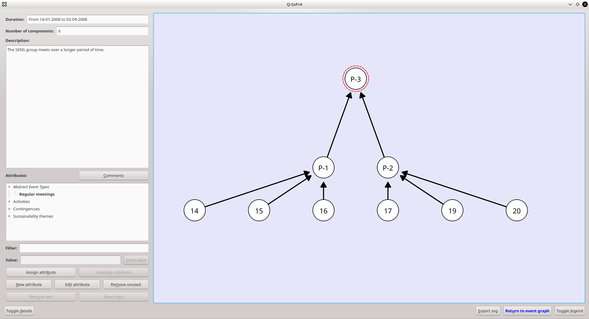
In the screenshot above, we are inspecting the hierarchy of abstract event “P-3”, which consists of two other abstract events “P-1” and “P-2”, which, in turn, each consist of three incidents (P-1: 14, 15, 16, and P-2: 17, 19, 20).

In this screen, we can select all visible events individually. As you can see, we again have the attributes tree available to the left of the screen, and we can assign attributes in the same way we would in the Event Graph Widget. Hierarchy graphs are thus the third ‘place’ where you can assign attributes to incidents (and events).

Other interactions with attributes

Of course, assigning attributes to incidents is not the only type of interaction with attributes that we need. Occasionally, we will want to edit the name or the description of an attribute, which can be done by selecting the attribute in the attributes tree, and clicking the Edit attribute button. This will simply open the dialog that we have seen before (when creating a new attribute), but with the details of the currently selected attribute already filled in.

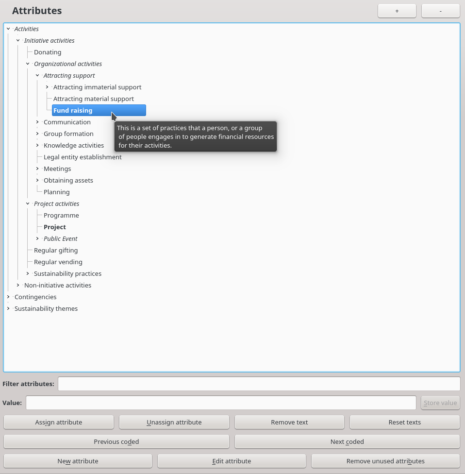
If we want to unassigning an attribute, we just select it in the attributes tree, and click the Unassign attribute button. We can also remove all attributes that are not currently being used by clicking the Remove unused attributes button.

I did not include the possibility to simply remove an attribute by clicking some kind of delete button. I thought that having this option is risky, because you might delete an attribute that you assigned to some other incident, for good reasons, that you have forgotten about. The only way you can thus get rid of attributes for good is by unassigning them from all incidents, and then clicking the Remove unused attributes button.

If there are fragments of ‘raw’ texts associated with the attribute, we can either select one of these fragments and click the Remove text button to remove an individual fragment, or we can simply click the Reset texts button to remove all fragments associated with the selected attribute (of course, this will only remove fragments that are associated with the combination of this attribute and the currently inspected incident). Any fragments of ‘raw’ text associated with an attribute will also be removed when you unassign the attribute.

We can also navigate incidents via attributes, by selecting an attribute, and clicking the Previous coded or the Next coded button, which will jump to the previous/next incident that was assigned to the selected attribute (or one of its children).

One other thing you’ll notice in the screenshot above is the tool tip that is displayed when you hover your mouse over an attribute in the attributes tree. The tool tip will show the description that you gave the attribute, making it easy for you to read the description without having to open another dialog.

Attributes in tables

There are a few other widgets in which attributes appear. These are tables that, for your convenience, present information that we have already seen in a somewhat different form. For example, in the screenshot below you see a table of attributes, the incidents they were assigned to, and the fragments of ‘raw’ texts associated with them.

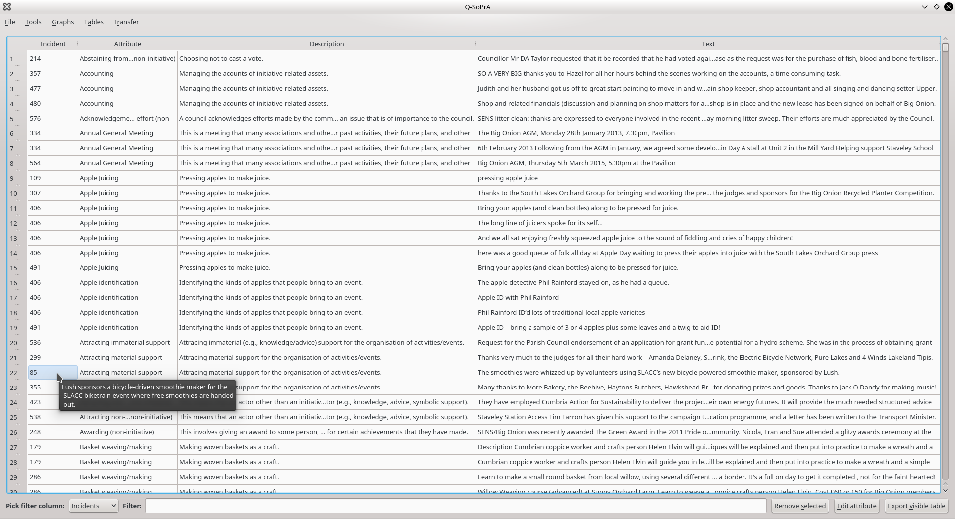
This particular table is mostly useful for a comparison of the various fragments of ‘raw’ text that are associated with an attribute. Based on such comparisons you can make decisions about, for example, the appropriateness of the name and description that you assigned to a given attribute. This is particularly useful in more grounded approaches to coding, where you will be revising your coding scheme (or, in this case, attribute scheme) repeatedly as you progress with your study.

In this table, incidents are identified by a number that corresponds to the order in which incidents appear (this is used as the primary way to identify incidents to the user throughout Q-SoPrA). Indeed, this number alone won’t tell the user very much, but as the screenshot above demonstrates, the description that was given to incidents can be revealed by hovering the mouse cursor over them.

It is possible to filter this table by using the filter field below the table. You can apply this filter to any of the visible table columns. The table can also be sorted by double clicking one of the column headers, and the order of columns can be changed by dragging columns to another place. Fragments of text can be removed by selecting a row in the table and clicking the Remove selected button. Attributes can be edited by selecting a row in the table and clicking the Edit attribute button. Finally, the table currently being shown can be exported by clicking the Export visible table button.

Another table in which attributes appear is shown in the screenshot below. In this case, the table shows attributes, the incidents that they were assigned to, and the values that were given to the attributes. The screenshot shows an example where I am inspecting an attribute that I used to map projects to which the activities recorded in incidents are related. To do this, I simply created an attribute called project, and I gave values to the attribute to indicate which project a given incident (activity) belongs to.

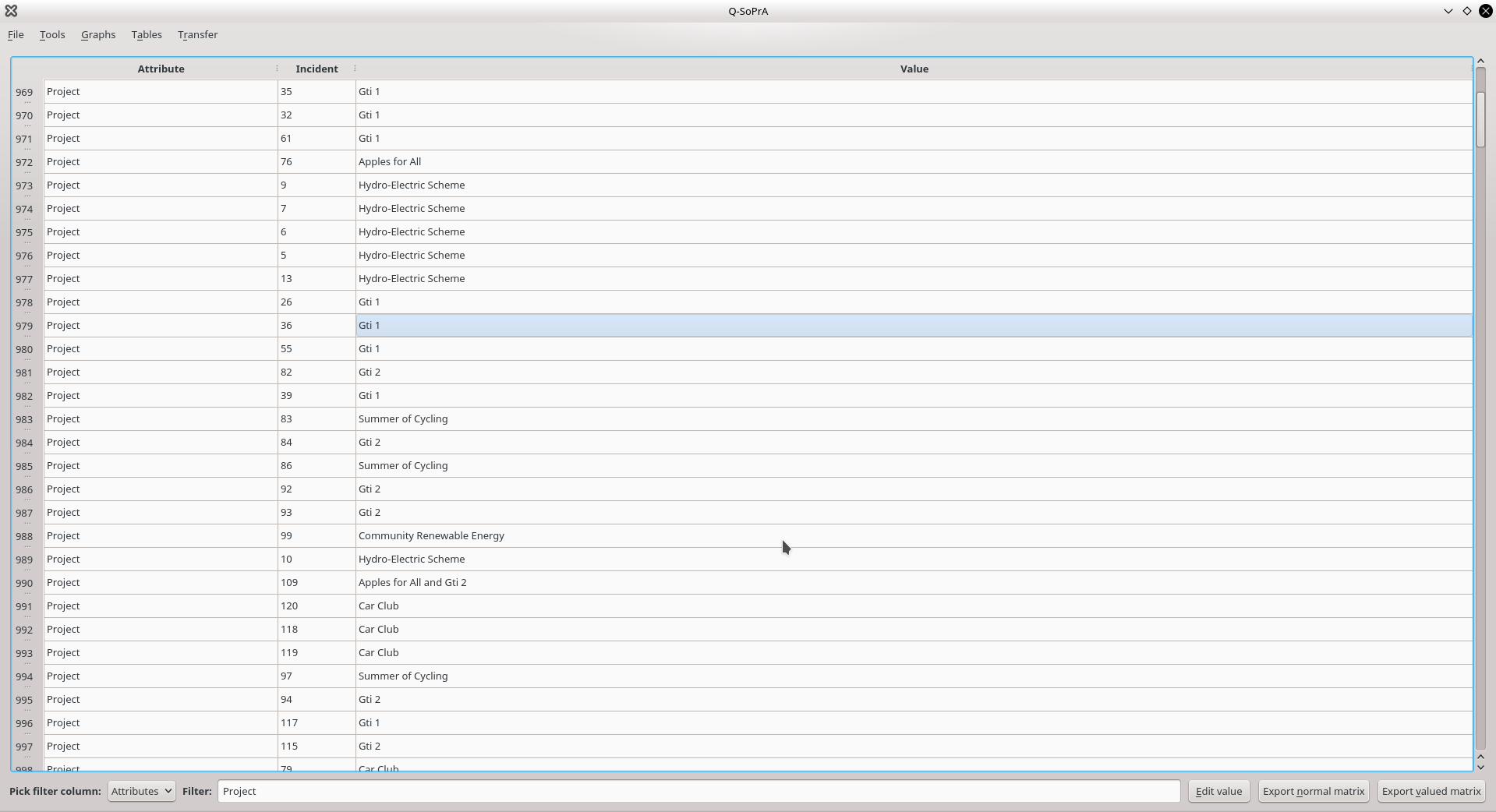
Like the previous table, this table can be filtered. Values that were assigned to attribute-incident combinations can be changed in this table by clicking the Edit value button. It is also possible to export a matrix of incident-attribute combinations. The exported matrix will be an incidence matrix, where the incidents appear in the rows, and the attributes appear in the columns. If you choose to use the Export normal matrix option, the cells of this table will show a 1 if the corresponding incident-attribute combination exists, and a 0 if it doesn’t. If you choose to use the Export valued matrix option, the cells will instead show the values that were assigned to incident-attributes combinations, wherever these are available. If no value was given, then the table will again show either a 1 or 0 depending on whether the corresponding incident-attribute combination was observed.

The final table I will discuss here is the one shown in the screenshot below. This is actually not a table in which attributes appear. Instead, it is a table that shows all incidents that do not have an attribute assigned to them. When you are coding a large data set, you are likely to at some point overlook something. For example, you may have inserted a new incident somewhere in your data set at some point, but you have forgotten to assign attributes to it. The table shown below makes it easier to spot any incidents that you may have forgotten about. In the example offered in the screenshot, the incidents shown are simply the incidents that I haven’t gotten to yet in the coding process.

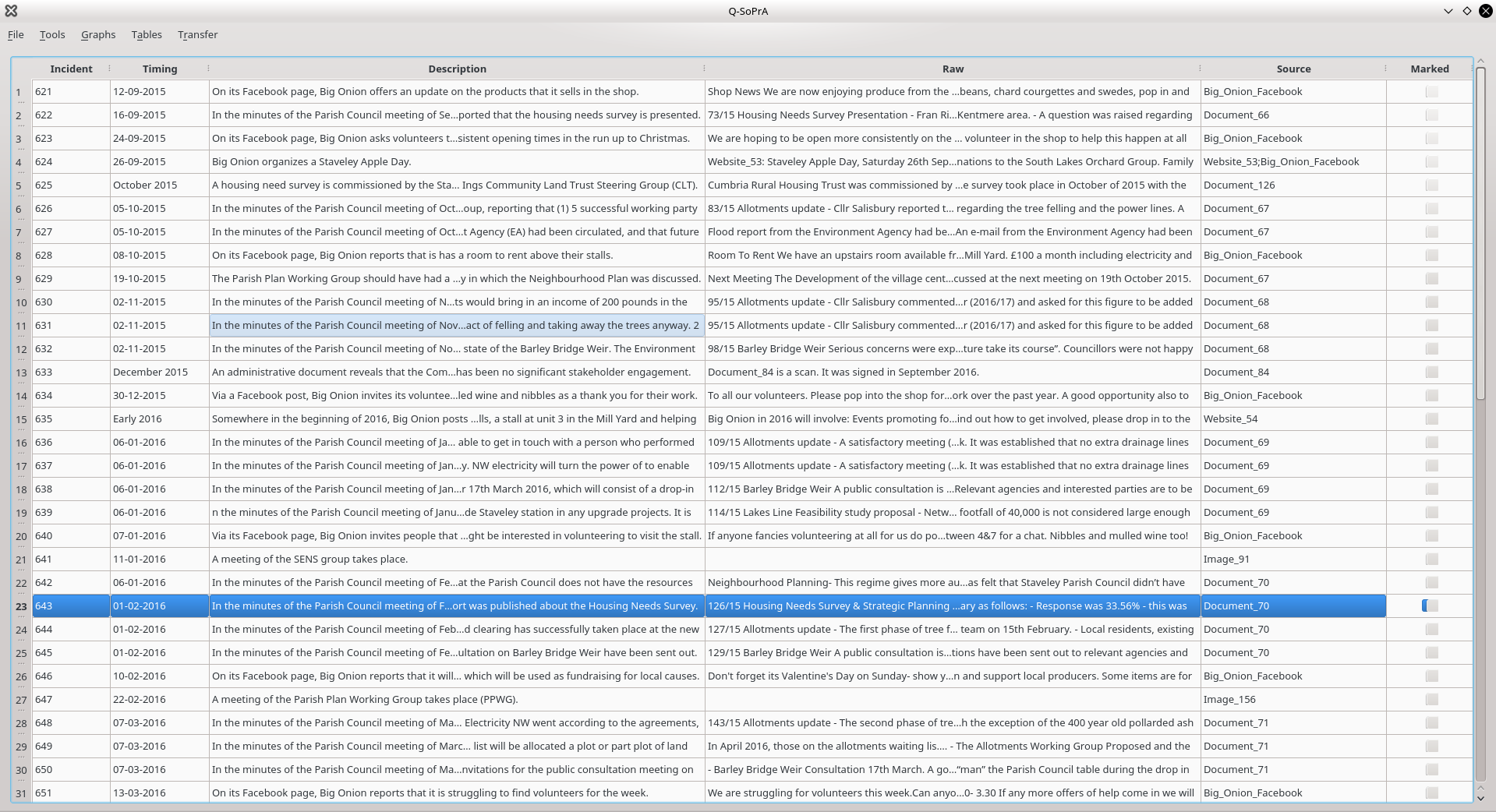
This table has something special, which is the last column of the table, called Marked. In Q-SoPrA all incidents can be marked, which simply makes it easier to find them back when using one of the coding widgets (in these widgets, you have the possibility to jump back and forth between incidents that are marked, skipping all other incidents). In this table, you can mark an incident by clicking its corresponding check box in the last column.

Attributes in visualisations

So, now we get to the last major part of this post, which is about how to use attributes in visualisations, which can be one step in your analysis of the data.

Attributes in event graphs

We have already seen the Event Graph Widget and how we can assign attributes to incidents/events there. Attributes can also be used to manipulate the visualisation of event graphs. One thing we can do is to create modes in the network based on attributes. In Q-SoPrA, a mode can be understood as a special identifier for nodes in the event graph (modes also appear in network graphs, but this is yet another topic that I will need to discuss in a future post). Any node (incident or abstract event) in the event graph can only have one mode at a time. What mode a given node belongs to is made visible by giving it a distinct colour.

In order to achieve this, the user has to create a mode. This can be done from the legend menu (see screenshot below). In the screenshot the legend is currently empty, because no modes have been created yet. A new mode can be created by clicking the Create mode button (in the bottom-right area of the screenshot). This will open a dialog with the attributes tree, as well as a few buttons that can be used to choose a colour for the mode (colours can be chosen for the nodes and for the labels).

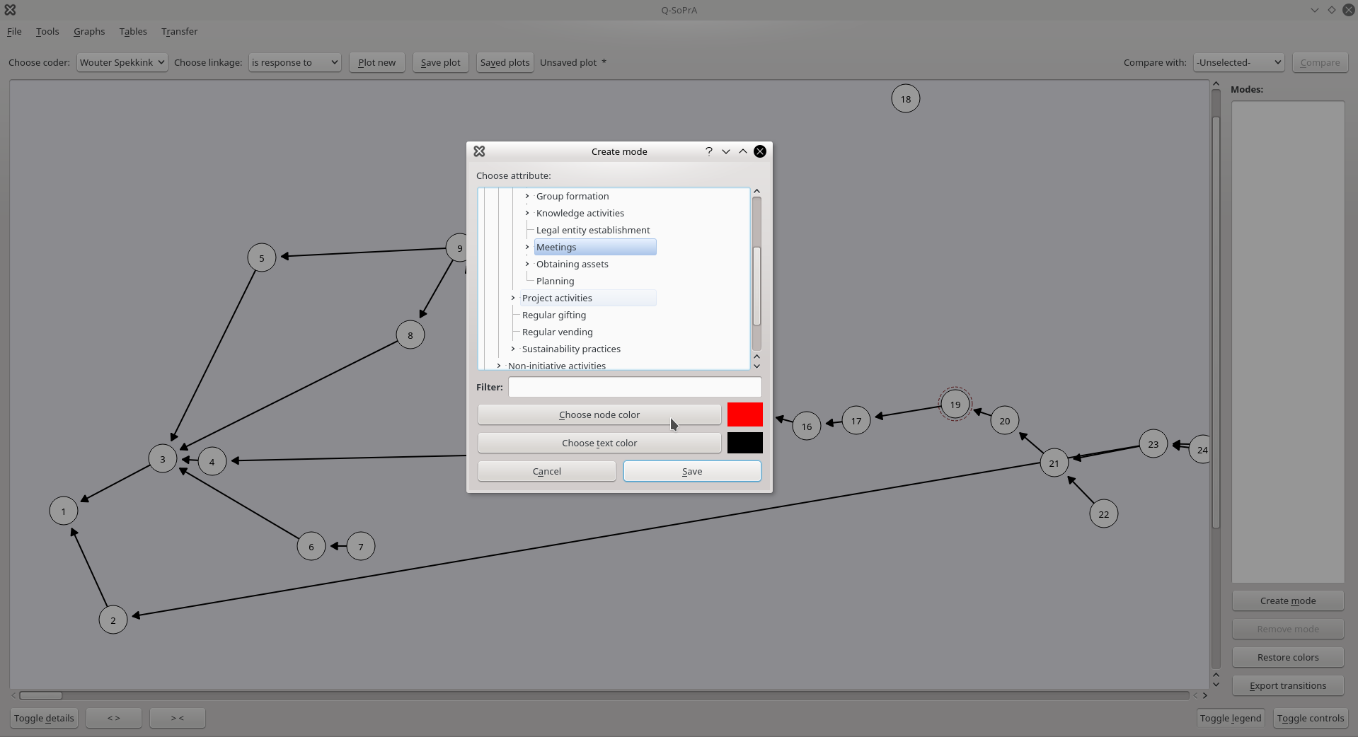
After choosing an attribute and the colours to be associated with it, we can save the new mode. Q-SoPrA will immediately identify all nodes in the graph that were assigned the selected attribute, or one of its children. I emphasise the last bit, because it is important to realise that modes in the event graph are inclusive in the following sense: A mode is identified by an attribute, as well as by all children of that attribute. Thus, in the screenshot below, all the red coloured nodes can be understood as incidents in which some kind of meeting took place, without specifying what type of meeting we are referring to. A label identifying the newly created mode will also be shown in the legend, to the right of the screen.

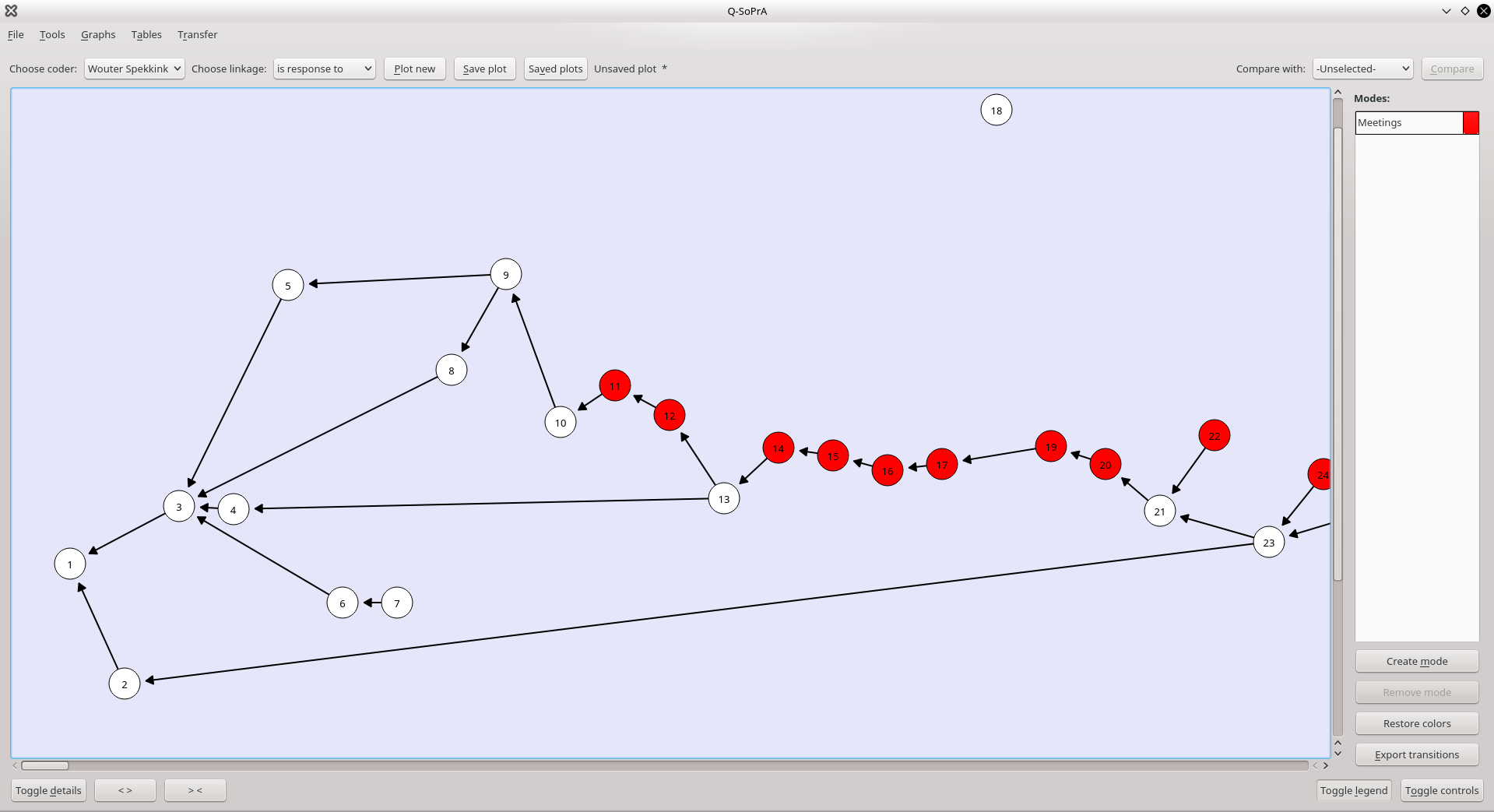
Modes are, in a sense, also hierarchical. In deciding what mode an incident or abstract event should be assigned to, Q-SoPrA will always work its way from the top of the list of modes (the legend) to the bottom. Any modes that appear near the bottom of the list will overrule modes that appear above them. For example, In this case, we could add an additional mode that refers to a more specific kind of meeting (a child of the Meetings attribute).

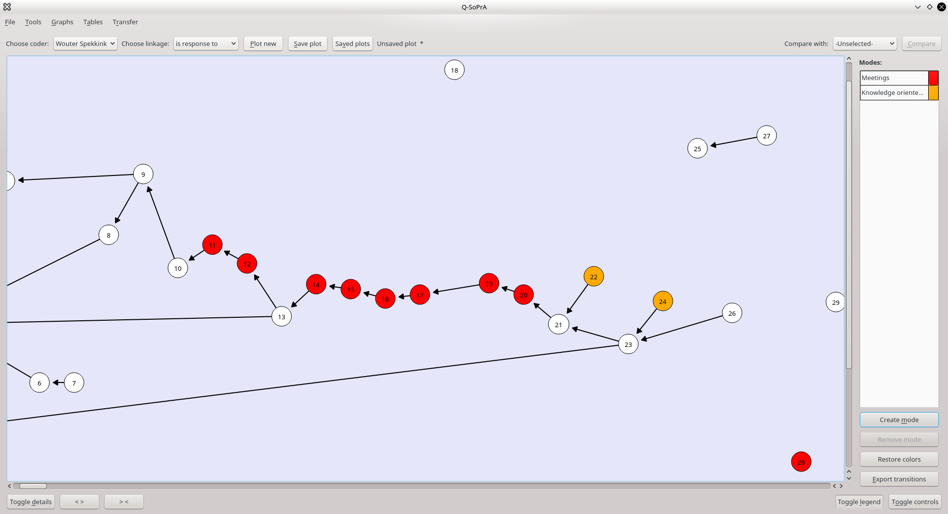
In the screenshot above, you will see that two nodes have been switched to another mode (incidents 22 and 24). In this case, the attribute Knowledge-oriented meetings overruled the attribute Meetings in deciding which mode should be assigned to these incidents.

So what happens if we add a mode that is associated with a parent of the Meetings attribute, rather than a child? Let’s test this by creating a mode based on the Organizational activities attribute, which is the parent of the Meetings attribute.

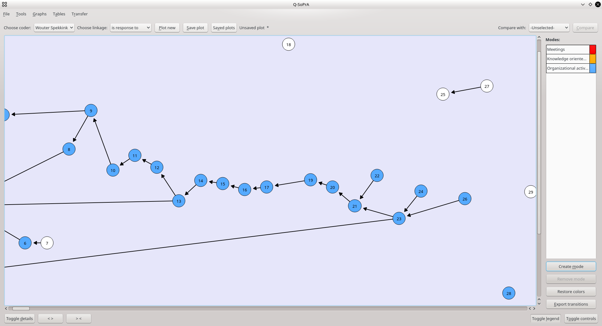
As you see in the screenshot shown above, this causes the earlier created modes to be overruled. Imagine that, at this point, we realise that we have made a mistake; that it was never our intention to overrule our first two modes. We can easily recover from this situation by selecting the last mode we created, and clicking the Remove mode button. This will remove the mode from the event graph, and Q-SoPrA will automatically reassign the earlier created modes, basically reverting the graph to the version we saw earlier.

I plan to make playing around with the modes even easier, by adding the option to move modes up or down in the hierarchy. This will be implemented in a future version of Q-SoPrA.

These modes are not just for visualisation purposes. One feature of Q-SoPrA that makes use of modes is the creation of transition matrices. These matrices show how often an event of a given mode has a relationship to an event of another given mode. Making such matrices can tell you a lot about how different types of events in your graph tend to be related. For example, it can give you crude measures of how likely an event of a given type is to be followed by various other types of events.

In the screenshot below, I have assigned modes that cover nearly all of the incidents visible in the current screen.

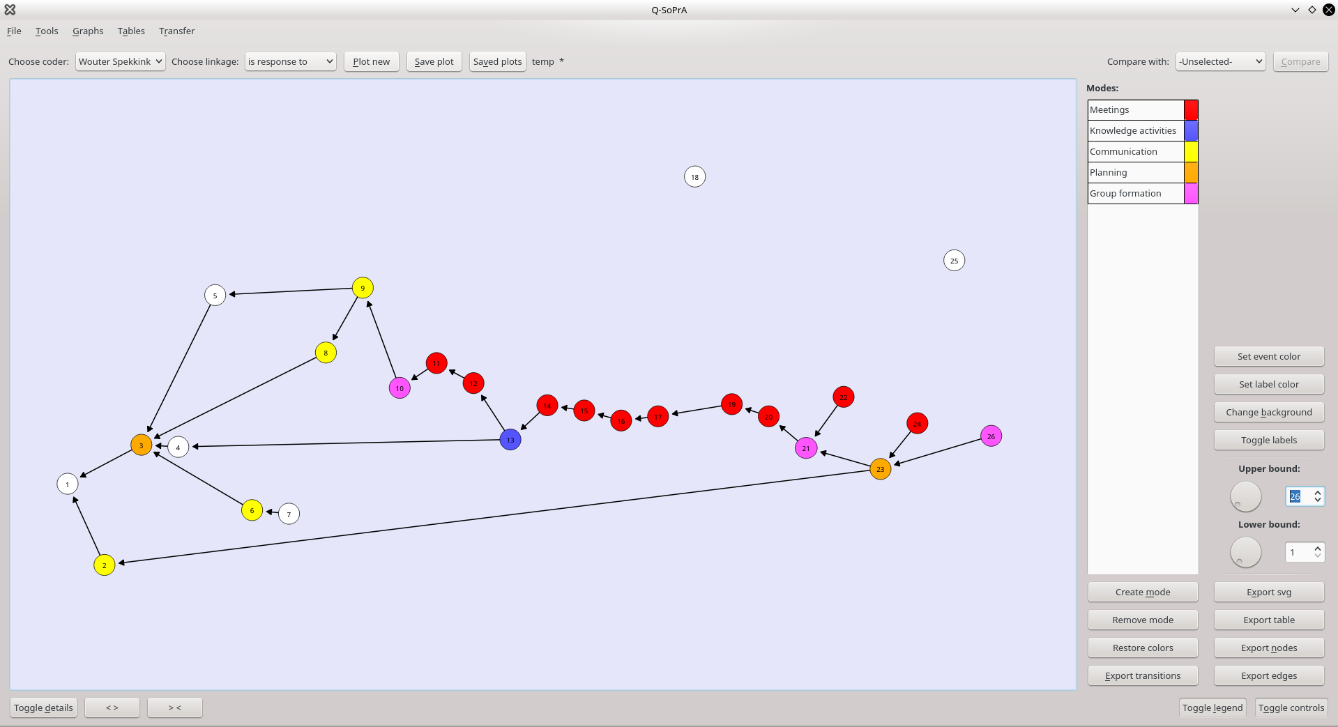
What I can do now, is to click the button Export transitions. This will open a new dialog (shown below), where I can choose what kind of transition matrix I want to export.

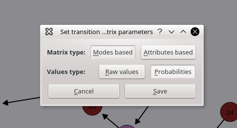
Now, the first two options shown here (modes vs. attributes) require a bit of explanation. In the above, we have learned that any incident can have only one mode at a time. However, an incident can of course have multiple attributes, and sometimes we will want to take all attributes into account when calculating transitions, rather than taking into account only the currently assigned modes. This is basically what you can do by selecting the Attributes based option in the dialog shown above. In this example, we’ll go with the Modes based option instead.

The other two options are much more straightforward: You can either (1) export a transition matrix with the raw counts of the observed transitions, or (2) export a transition matrix where these counts were divided by the row marginals (the number of times the source event of the transition appears), which converts the value into a crude measure of probability. We’ll go with the latter option.

Q-SoPrA will now ask us what we want to name our file (which is a csv-file), and where we want to store it. After saving the file, we can open it with a spreadsheet editor, like LibreOffice Calc or Microsoft Excel. In the screenshot below, I show the matrix I exported from the last version of the event graph. I slightly edited the matrix before making the screenshot, adding bold fonts to the rows and columns, making the final row and column italic font, and formatting the transition probabilities to show 4 decimal numbers.

As you will see below, the transition matrices that Q-SoPrA exports always contain a column with the row marginals. Thus, if you export a transition matrix with the raw counts, then you can easily calculate probabilities yourself by dividing these counts by the row marginals.

In addition to the row marginals, the transition matrices will always include a row with the number of times the different event times participated in transitions (as the source event).

One of the things we see in this table is that, based on the observed event graph (which I filtered to only show the first 26 incidents), there is a probability of 0.6 that an event of the mode Meetings followed an event of the same mode. Given that the row marginal for this mode is 10, this must mean that this particular transition was observed 6 times (6/10 = 0.6). We also see that it is as likely that an event of the mode Planning follows an event of the mode Communication as it is to follow an event of the mode Group formation (0.5 probability in both cases). You can do a visual check of our screenshot of the event graph to confirm this.

Of course, with this small number of observations, these numbers are unlikely to be very meaningful. However, I hope the example demonstrates how transition matrices can be useful in summarising patterns in your data. Patterns like these will be especially hard to detect without transition matrices once you start considering larger numbers of incidents/events.

Attributes in occurrence graphs

The last thing I will discuss here is the use of attributes in the creation of Occurrence Graphs. Occurrence graphs visualise which attributes co-occur at which points in time. Attributes can co-occur, for example, because they are assigned to the same incident, because they are assigned to incidents/events that were grouped in the same abstract event, or because they are assigned to incidents that occurred in parallel (incidents and events can be made parallel in the Event Graph Widget).

Occurrence graphs are basically a slightly adapted variant of Bi-Dynamic Line Graphs (BDLGs), which, I should emphasise, is not a type of graph I came up with myself (see the link to my earlier post on BDLGs to learn more about them). I will discuss occurrence graphs in more detail in another post, and only touch on some basic details here.

In an occurrence graph, attribute-incident (or attribute-event) combinations are visualised as nodes. The position of the nodes on the horizontal axis is based on the chronological ordering of the incidents/events (this ordering can also be matched to that of customised event graphs). In the occurrence graphs edges only appear between nodes that refer to the same attribute, and they always point to the next attribute-incident (or attribute-event) combination in which that attribute occurs. When attributes co-occur, their attribute-incident (or attribute-event) nodes appear at the same coordinate of the horizontal axis.

Occurrence graphs can thus be understood to show the ‘history’ of one or more attributes’ appearance/involvement in the process of interest. Imagine that you have a set of attributes that identify different actors that participate in the process your are studying. An occurrence graph can give you a quick overview of (1) when these actors were active, (2) how frequently they were active, and (3) which actors tend to be involved in the same incidents/events. For another example, imagine that you have a set of attributes that identify different types of activities that occur in incidents/events. An occurrence graph can give you a quick overview of (1) when these activities occur, (2) how frequently these activities occur, and (3) which activities are typically carried out in combination.

Q-SoPrA has a separate widget for the visualisation of occurrence graphs. An occurrence graph is built by adding attributes one by one, as I will demonstrate in the example below.

In this example, I will use an occurrence graph to study a specific issue of interest me. The data set that I use in this example records the emergence and development of a community sustainability initiative, somewhere in the UK. One of the ambitions of the initiative is to stimulate people in the community to adopt more sustainable practices (that is, what the members of the initiative understand to be sustainable practices, like growing your own food, commuting by bicycle rather than by car, crafting your own products from locally sourced materials, and so on). I have various attributes that refer to these different kinds of practices, and these all share a parent that I called Sustainability practices. What I want to know is what other activities the members of the initiative use to promote sustainable practices. One way to do this is to study what other activities the Sustainability practices co-occur with.

The first thing that I do is to add the Sustainability practices attribute to my occurrence graph. As was the case with modes in the event graphs, this will create nodes for all incidents that have the Sustainability practices attribute assigned to them, or one of its children.

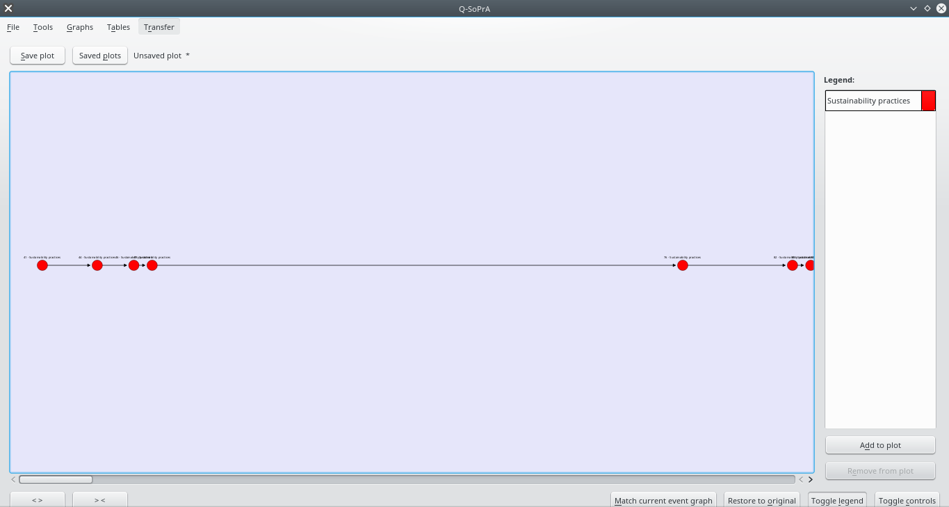
Q-SoPrA will plot the nodes that refer to the same attribute on a straight line, where the position of the nodes on the horizontal axis respects their position in the chronological order of incidents. A small portion of the graph is shown in the screenshot above. Not terribly exciting, is it?

Let’s add some other attributes. One of the things that I learned is that members of the community sustainability initiative I studied like to make use of workshops to teach other members of the community certain skills associated with Sustainability practices. I therefore add an attribute that I used to capture the occurrence of workshops, called Initiative workshop.

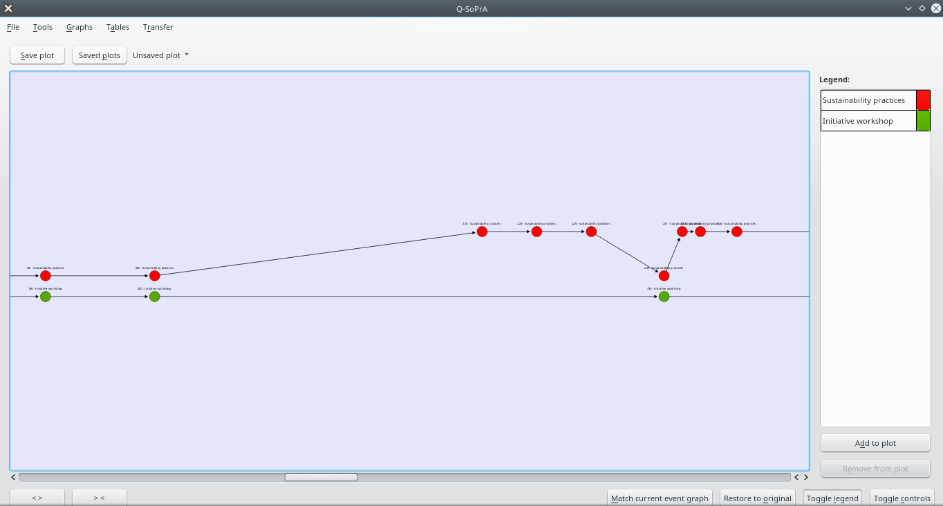
There are immediately quite some co-occurrences that appear in the graph (see the screenshot above for a fragment of the graph). I made sure that Q-SoPrA initially plots all attributes-incident combinations on their own line, and that combinations that co-occur appear close to each other, so that co-occurrences are more pronounced (of course, you can move the nodes around a bit to adapt the visualisation).

What I unfortunately cannot show you without flooding this post with screenshots is that the occurrence graph shows that workshops occur quite often, but mostly in a particular episode of the process. Thus, it is interesting to explore some other types of activities that might be used to promote Sustainability practices to see if these are perhaps bound to certain episodes as well. The next attribute I’ll add is Competition, which captures those occasions where members of the community sustainability initiative organised some kind of competition to engage people in certain practices (e.g., cycling competition, a competition for who builds the nicest planter, and more).

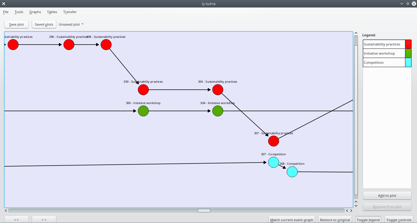
The screenshot above shows just a small segment of the graph, but it shows one example where a Competition co-occurs with Sustainability practices. Actually, these co-occurrences appear in various parts of the graph, but overall they appear more sporadically than those of Sustainability practices and Workshops.

For this example, let me add just one more attribute. In this case I added the attribute Door-to-door advice, which is an activity in which members of the initiative went door-to-door in their community to provide community members advice about energy saving measures that can be taken at home.

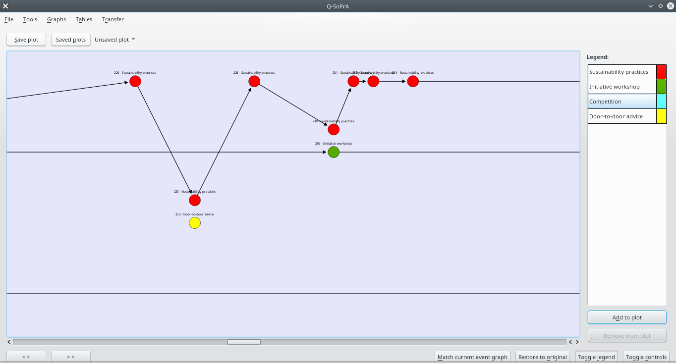
As the screenshot above shows, I apparently only used this attribute once. There are no edges going into, or out from the yellow node shown in the screenshot, indicating that the node only appears once in this graph. The fact that this activity only occurs once is easily explained. The activity was carried out as part of a project for which the community sustainability initiative obtained funding, and which was dedicated to implementing and promoting energy saving measures in the community. As part of the project, some members of the initiative were trained to provide personalised energy advice, and these members went door-to-door in their community. Of course, this is a relative expensive operation for a small initiative, and it is not something you would expect to happen on a regular basis. The organisation of workshops, for example, typically requires lower investments of time and money, which perhaps makes it a more attractive type of activity for the initiative to make use of.

If we really want to make a more in-depth analysis, we would of course not stop here, and we would probably repeatedly go back and forth between our underlying data, the occurrence graph, and other visualisations and tools, but I think this small example gives you a basic idea of what you can do with attributes and occurrence graphs.

There is just one other thing I want to demonstrate. If you are familiar with CAQDAS, then you are probably also familiar with the concept of co-occurrence of codes. Basically, the occurrence graphs visualise a certain type of co-occurrence, a type that is sensitive to temporal order. However, it can also be useful to just have an aggregate measure of co-occurrence, like you would have in most CAQDAS. After creating an occurrence graph in Q-SoPrA it is possible to export a (co-)occurrence matrix that records aggregate measures of (co-)occurrence. The screenshot below shows an example of such a matrix.

The diagonal of the matrix simply shows how often a given attribute occurs overall. The other cells of the matrix show co-occurrences of the attributes associated with the corresponding rows and columns. This matrix basically gives us similar information to the occurrence graphs we studied earlier. For example, it shows that, when workshops occur, they typically co-occur with sustainability practices. It also shows that workshops were used more often than competitions, and that door-to-door advice occurred only once. Of course, what the matrix does not show us is when in the process all these activities (co-)occurred, so with the matrix we do loose some potentially relevant information.

Closing comments

There are of course more things that can be done with attributes. It is relatively easy to export data from Q-SoPrA, and to import it into some other software package for further analysis. For example, you could try to import the incidence matrix of incidents and attributes into some network visualisation tool, and make a network graph of what attributes are related to what incidents, giving you an overview that is otherwise perhaps hard to obtain.

It is very likely that I will also be adding additional features to Q-SoPrA over time. For now, I hope that the above demonstrates how attributes in Q-SoPrA can support in the analysis of social processes.