Relationships in Q-SoPrA

Introduction: Process and structure

As the name suggests, Q-SoPrA (Qualitative Software for Process Analysis) is focused first and foremost on the qualitative analysis of social processes. However, I invested a lot of time and energy in also creating features that can be used to study how these processes relate to structures. In my opinion, this is a somewhat obvious thing to do, since so many social theories posit some kind of relationship between process and structure (often couched in terms of agency and structure. I can use my own application of Q-SoPrA as an example. I am currently using Q-SoPrA in a study that, conceptually, builds on Schatzki’s concepts of social practices (in short, organised doings and sayings) and social arrangements of people, artefacts, places, and other types of entities. I use event graphs to reconstruct practices as networks of activities (Schatzki also writes about chains of action in this context), and I use more traditional network graphs to reconstruct arrangements as networks of relationships between entities. One aspect of my investigation is to study how unfolding practices relate to (changes in) arrangements.

I believe that many other theoretical perspectives are compatible with Q-SoPrA, although Q-SoPrA probably fits best with perspectives that assume primacy of process over structure (see Rescher). In other words, Q-SoPrA connects best with the assumption that (social) life is essentially a flux, and that the emergence and persistence of structures are generally accidental properties of processes, even if those these accidental properties can be widespread (and I think they are). This assumption can be opposed to the assumption that reality is fundamentally structural, and that change and development are accidental properties of structures.

I should perhaps add that, in my view, this does not necessarily mean that processes should always have priority in the explanation of social phenomena. I think it is perfectly reasonable to assume that structures emerge from process, but are then capable of shaping or inducing processes in radical ways, and are therefore of great explanatory value, depending on the specific research questions being asked.

That being said, from a process perspective it would then still be obvious to also ask the question what processes lead to the (re)production of that structure.

So how does Q-SoPrA assume primacy of social process? Well, by using incidents as indicators for relationships (although it is of course equally possible to think of incidents as enactments of relationships without changing the general approach). More specifically, Q-SoPrA allows you to define relationships (I discuss the details below), and then assign these to incidents in the same way that you would assign attributes. This also creates the benefit that it becomes possible to study networks of relationships that were indicated by incidents in a particular episode of the process, thereby providing a rudimentary way to look at changes in networks of relationships over time, as I discuss further below.

In the past, I used to do something similar by assigning actors to events (as attributes), and then looking at the co-participation (or co-affiliation) of actors in events over time (also see my post about bi-dynamic line graphs). Two important limitations of this approach are that (1) co-participation is basically an abstract summary of many different ways in which actors can be related to each other through events, and (2) not all relationships that are indicated by events are necessarily captured by their co-participation. To offer an example of the first limitation, imagine that we have two events in which the same pair of actors interacted with each other, but that in one event the interaction concerned the joint organisation of an activity, and in the other event the interaction concerned one actor providing financial support to the other actor. If we simply model both occasions as co-participation, then we lose the ability to distinguish between the two situations. To offer an example of the second limitation, imagine that we have an activity in which an individual is acting as a representative of a certain group. If we want to capture this fact as a membership relation, it would be awkward to capture it as co-participation of the individual and the group in the activity. Instead, it would make more sense if we could simply define a membership relationship, and say that the activity is an indication of the individual being a member of the group.

The way I implemented relationship coding in Q-SoPrA is basically an attempt to take away these limitations. In addition, I made sure that Q-SoPrA is able to visualise networks of relationships that have multiple modes (for an introduction into two-mode networks, see this blog post; Q-SoPrA allows you to define more than two modes), and multiple types of relationships. Parallel edges (multiple edges between the same pair of entities) are drawn with curved lines to make sure that multiple types of relationships can be visualised in one graph. In addition, it is possible to perform multi-mode transformations to infer ‘latent’ relationships from observed ones. I will explain all of this in detail in the remainder of this post.

Before I proceed, I should make the note that the example data set that I use below is based on a narrative that Peter Abell provided in one of his papers on Comparative Narratives. Abell’s theory and method of Comparative Narratives are major sources of inspiration for the ideas implemented in Q-SoPrA.

The relationships widget

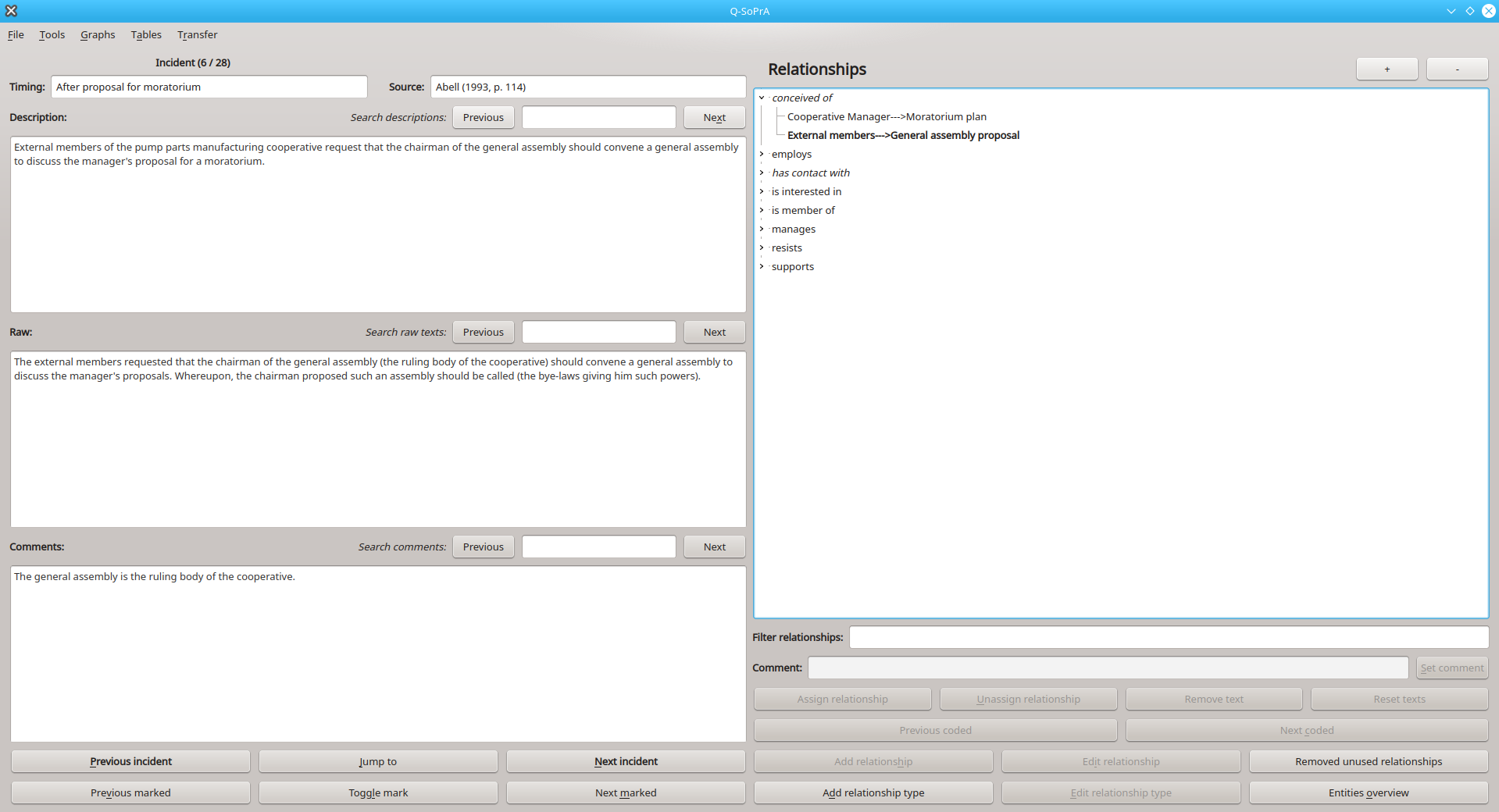
In the screenshot below you see what the relationships widget looks like. If you’ve seen my earlier post on attributes in Q-SoPrA, you’ll notice that the relationships widget and attributes widget look very similar. Each incident in the data set can be inspected individually, with the information available on the incident displayed in the left half of the screen. With the navigation buttons at the bottom-left you can go through the previous or next incident as they appear in the overall chronological order (which you set in the data widget), you can jump to the previous or next incident that is marked (incidents can be marked and unmarked with the Toggle mark button), or you can jump to a specific incident by using the Jump to button.

In the right half of the screen you will see a relationships tree (when you start a new data set, this tree will be blank). This tree works a bit different from the attributes tree. One important difference is that the relationship tree can only have two levels. The first level of the tree shows relationship types, and the children of each relationship type are instances of this type. As we can see in the screenshot below, we have two instances of the conceived of relationship type, one of which captures that the entity “Cooperative Manager” conceived of the entity “Moratorium PLan”, while the other captures that the entity “External members” conceived of the entity “General assembly proposal”.

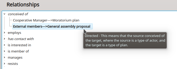
We can learn more about the definition of this relationship type by hovering our mouse over it (or hovering it over one of its instances). A tool tip with a description of the relationship will appear, as shown in the screenshot below. The description will always start with an indication of the directedness of the relationship, which may be set to Directed or Undirected. This is followed by the definition of the relationship that was created by the user.

The directedness of relationship types is also visualised in the labels that represent instances of that relationship type. As you can see in the screenshot below, the label of the two visible instances have a single arrow pointing from left to right, meaning that the relationship is directed from the entity on the left to the entity on the right. With undirected relationship types, there would be a double arrow pointing in both directions.

I assume that you are familiar with the idea of directedness in relationships (in the context of network analysis). If not, this probably means that you still need to familiarise yourself with the basics of social network analysis, and I would suggest taking a look at the book by Wasserman and Faust, which I think works great as an introduction, as well as an in-depth work of reference.

Defining relationship types

So how do we define relationship types in Q-SoPrA? This can be done by clicking the Add relationship type button. This will open a new dialog where the details of the relationship type can be written. The screenshot below shows an example of this, using the conceived of relationship type. As you can see, we can create a label for the relationship type, which is the label that is shown in the relationships tree. We are also required to offer a description of the relationship type, and we have to set its directedness. The same dialog will appear if you select an existing relationship type and click Edit relationship type in the relationships widget, but in this case the details of the existing relationship type will be shown in the dialog.

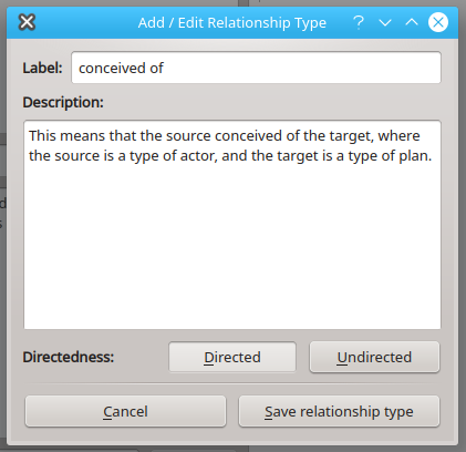
As you can see in the screenshot above, in the definition of this relationship type I have also indicated what types of entities can enter into this relationship (and in what role). In this case, I indicated that the source of the relationship should always be a (type of) actor, and the target should always be a (type of) plan. This implies that actors and plans are different types of entities in our data set, and in Q-SoPrA we can actually define different types based on attributes that we assign to entities. I’ll get back to this point further below.

Creating new relationships

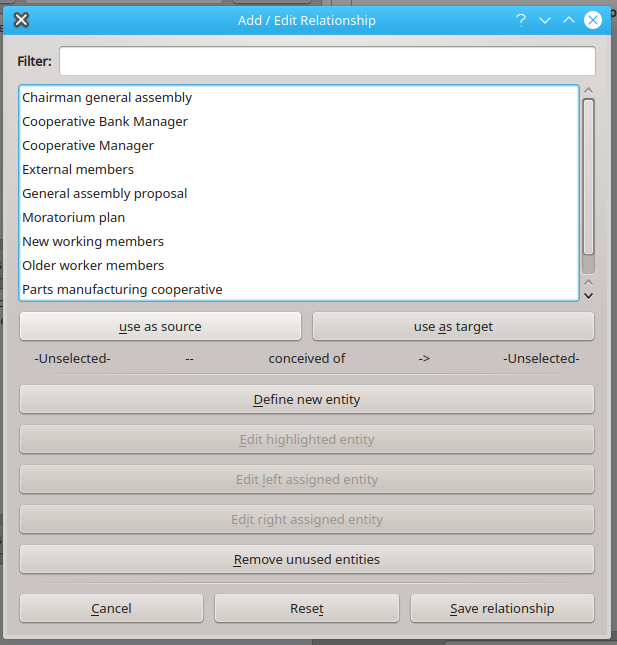
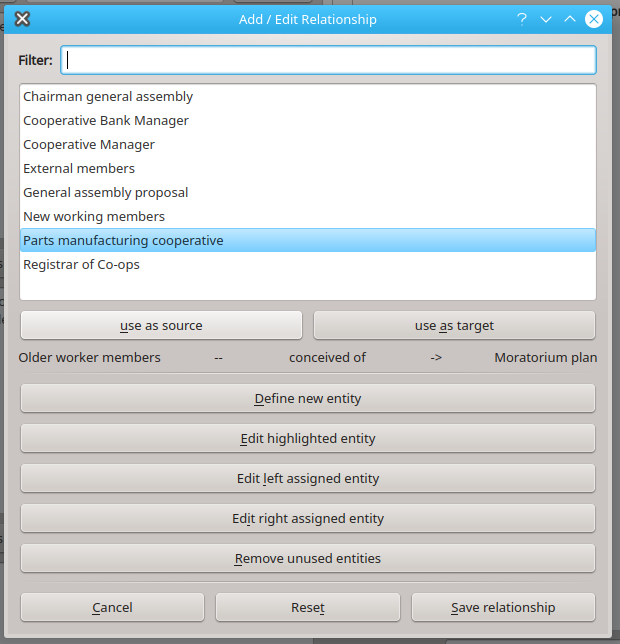
After we have defined a new relationship type, no instances of this relationship type will exist yet. For this, we have to explicitly create new relationships. This can be done by first selecting a relationship type in the relationships tree, and then clicking the Add relationship button. This will open another dialog (see below). In the dialog we see a list of entities (this list can be filtered with the Source filter), and several controls.

Defining a new entity

The list of entities will be empty if you have not defined any entities yet. Let us assume for a moment that this is the case. Before we can actually create a new relationship, we need to define entities that can enter in that relationship. This can be done by clicking the Define new entity button. This will open another dialog where a new entity can be created, as shown below. You are always required to provide a name and a description for your entity. In addition, we can use an attributes tree to assign attributes to the entity. This work almost exactly the same as assigning attributes to incidents, except that we cannot associate any ‘raw text’ with entity attributes.

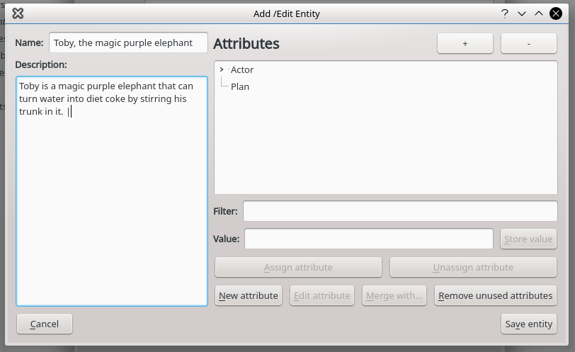
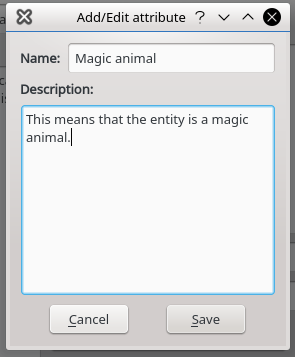
New attributes can be created in this screen as well. For this we would click the New attribute button. This will open yet another dialog (see below), but you’ll be pleased to know that we won’t open any other dialogs from here. The new dialog is a simple dialog where a label and description for the new attribute can be created. After creating the new attribute, it will appear in the attributes tree of the previous dialog. For this example, I have decided not to create the entity “Toby, the magic purple elephant” anyway, because it doesn’t really contribute anything to my case study.

Assigning entities to relationships

If we have defined at least two entities, we can assign them to the relationship that we are creating (in Q-SoPrA, entities cannot enter into a relationships with themselves). If you look at the screenshot of the relationships dialog below, you’ll see that under the list of entities, there are two buttons: use as source and use as target. Below these buttons you’ll see a description of the relationship as it is currently defined. When no entities have been assigned yet, in place of the Source and the Target, it will simply say “-Unselected-“. Entities can be assigned by selecting them in the list, and then clicking one of the use as… buttons. This will also change the description of the relationship (see below).

After we have assigned entities to our relationship, we can save it. It will now appear as one of the instances of the selected relationship type in the relationships tree. Each relationship can only be defined once. I should note here that undirected relationships with the source and target switched around are treated as identical. So, a relationship like Wouter<–has contact with–>Toby is treated as being identical to Toby<–has contact with–>Wouter.

Editing entities

In addition to defining new entities, we can also edit existing ones from this dialog. This can be done by selecting an entity in the list and clicking the Edit highlighted entity button, or by clicking the Edit left assigned entity or the Edit right assigned entity buttons to edit entities that were already assigned to the currently inspected relationship. This will open the same dialog that is used for defining new entities, but with the details of the selected entity already filled out.

Assigning relationships

Assigning a relationship to an incident does work the same as assigning attributes. In short, you select a relationship in the relationships tree, and then click the Assign relationship button to associate the relationship with the incident that is currently being inspected. It is also possible to associate a fragment of raw text (in the Raw field in the left half of the screen), by highlighting the text before clicking the Assign relationship button (this can also be done after the relationship is already assigned). If you want to disassociate a fragment of text from an assigned relationship you can either select this fragment of text in the Raw field, and then click the Remove text button, or you can click the Reset texts button, which will remove all fragments of text associated with the selected relationship and incident.

As with attributes, it is possible to navigate incidents via relationships that are assigned to them. This can be done by clicking a relationship, and then clicking the Previous coded or the Next coded buttons, which will jump to the previous/next incident that has the selected relationship assigned to it.

Filtering and commenting on relationships

I think it is likely that you’ll create quite a large number of relationships if you’re going to make use of the relationships widget. This means that the relationships tree quickly becomes heavily populated. By grouping relationships under different types, it should be possible to keep an overview relatively easily. However, often it will be easier to simply filter the relationships by using the Filter relationships field. For example, if you’re looking for a relationship that involves a particular entity, you can type the entity’s name in this field, and Q-SoPrA will filter out all relationships that do not include this entity.

You can also add comments to relationships. These comments are associated with the relationship itself, not with specific relationship-incident pairs. This is just like writing a comment/memo, but in this case the comment/memo applies specifically to a relationship. This can be achieved by selecting the relationship in the list, then typing the comment in the Comment field, and clicking the Set comment button afterwards.

Visualising networks of relationships

In the previous sections, I discussed how relationships can be defined, and then assigned to incidents. After you have identified relationships in your data, the more interesting thing to do is indeed to visualise them. I created the network graph visualisation widget for this purpose.

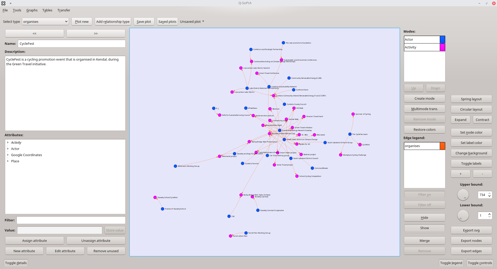
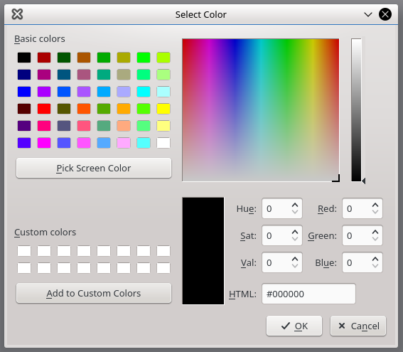
When you switch to this widget, it will initially be blank. To start plotting a network, you have to select a relationship type from a drop-down menu in the top left of the screen. In this menu, all relationship types that you have created are listed (see above). If you select one of them, you can then click the Plot new button. This will open a dialog that you can use to assign a colour to the relationship type you wish to plot (see below). By assigning different colours to different relationship types, we can distinguish between them in the visualisation. The colours belonging to different relationship types are listed in the legend, which can be opened by clicking the Toggle legend button at the bottom right of the network graph widget’s screen.

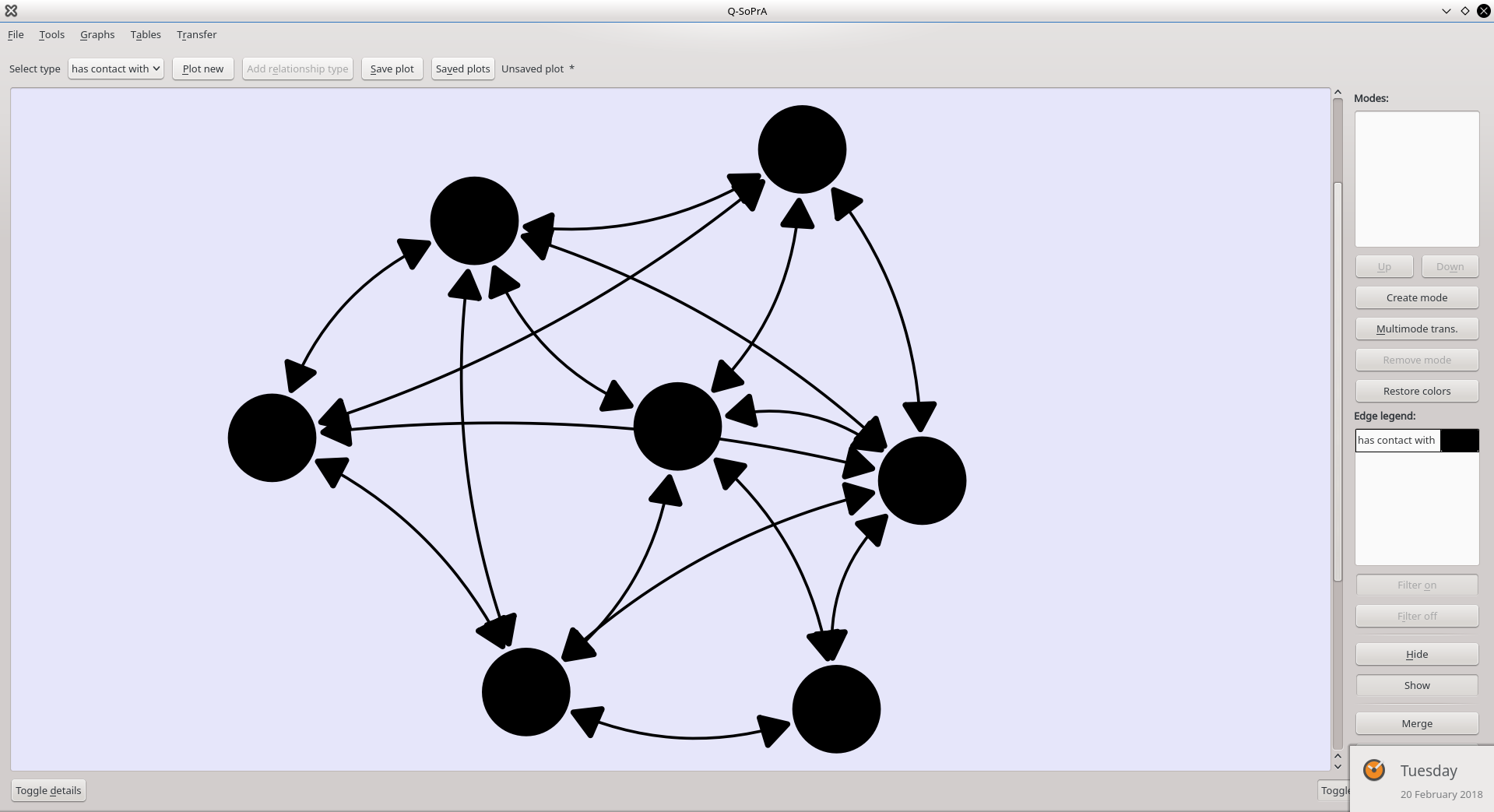
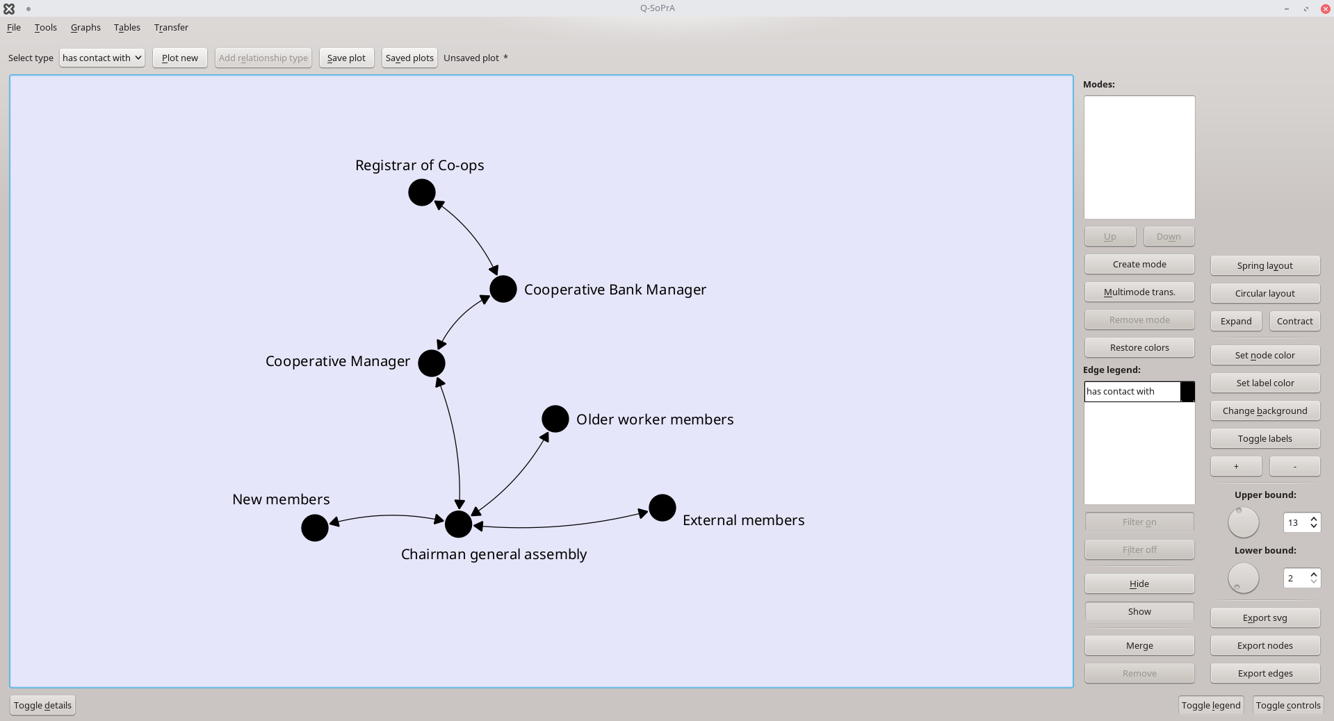
When you plot the network (I have chosen to plot the has contact with relationship, using the default black colour for the edges/relationships), it will appear in the draw screen (see below). The graph will initially just have a collection of unlabeled nodes (a selection of our entities) and the relationships between them. Q-SoPrA will always only show entities that are in a relationship that is currently visible (this also means that there can never be isolates in networks plotted by Q-SoPrA).

The graph layout

The default layout by Q-SoPrA is a ‘spring-like layout’. It is basically an intuitive layout algorithm that I quickly implemented as a temporary placeholder when I was creating this widget. However, with some improvements over time it actually turned out to function quite well, so I never bothered to find and use another algorithm to replace it with. I did add a second layout algorithm, which is the circular layout. As the name suggest, this will simply layout the nodes in a circle.

The circular layout does in fact do a little bit more than that. If you have modes assigned to your network (discussed further below), the nodes in the circular layout will be sorted by mode.

It is possible to expand or contract the layout by using the appropriate controls (these can be found in the Controls menu, which can be opened by clicking the Toggle controls button). It is possible to drag around nodes by clicking and dragging them with your mouse cursor. If you select multiple nodes, you can drag them around as a group by holding the CTRL button while clicking and dragging. I implemented very basic collision detection to make sure that nodes push each other away when they bump into each other.

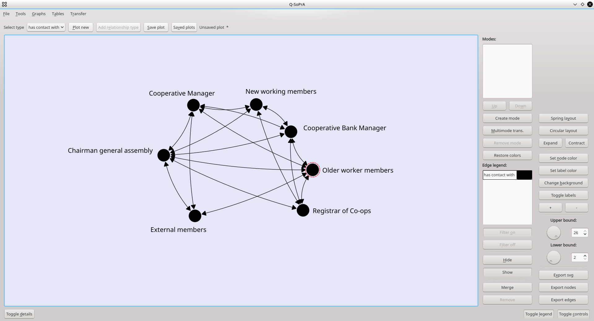
In our current plot, it is impossible for us to clearly identify our entities. We can improve the visualisation a bit by adding labels to the graph. This is also done from the Controls menu, where you will find a button Toggle labels, which can be used to show/hide node labels. Like the nodes, node labels can be dragged around individually by clicking and dragging them with your mouse cursor. However, wherever a node label is located relative to its ‘parent node’, it will always mimic the movements of that parent node. This allows you to change the position of the labels to make the graph more readable (see below).

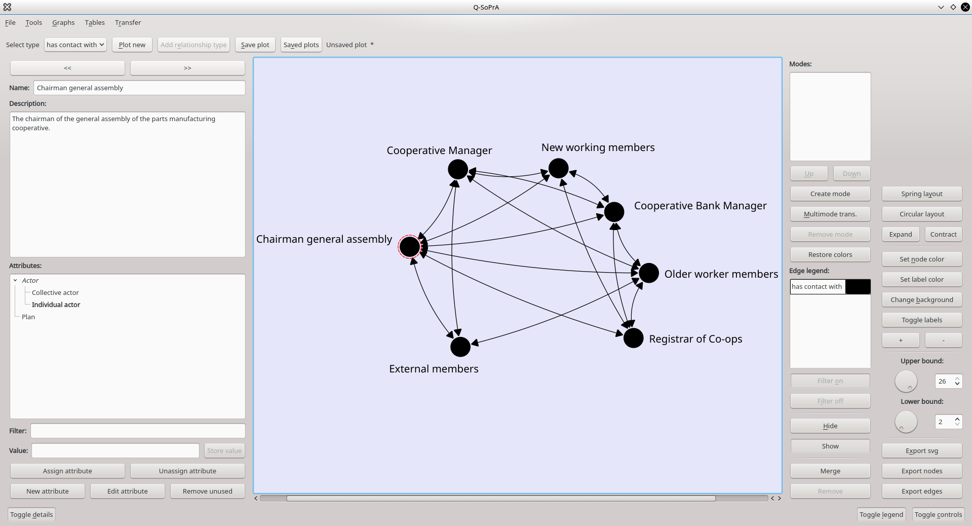
There is also another way to see more details about the nodes. We can hover our mouse cursor over nodes to see a tool tip with their name and description, or we can open the Details menu (by clicking the Toggle details button) to see the details we have available on the nodes that are currently selected, including attributes assigned to them (see below).

Filtering relationships

The network we are currently visualising is quite dense. This is because nearly all actors have been in contact with each other at least once in the process. In this visualisation, all the moments that we observed that actors were in contact with each other are aggregated. It can be interesting to filter out certain episodes in the process, to see what the network looked like during a specific episode of the process.

Q-SoPrA does this in a rudimentary way, by allowing you to set upper and lower bounds for the incidents that should be included in the visualisation. Indeed, the incidents themselves are not directly visible in the graph, but the relationships that were assigned to incidents are. By changing the upper and lower bounds in the Controls menu, we can thus manipulate the visualisation to only show relationships that were assigned to incidents that fall within those bounds. In the screenshot below you can see that our network becomes sparser if we filter out some of the later incidents in our data set.

Filters can also be disabled for individual relationship types. This can be done by selecting the relationship type in the legend, and clicking the Filter off button. This means that all relationships of this type will be shown, no matter what bounds you have set in the Controls menu, effectively allowing you to filter some relationship types, while keeping others fixed. To set the filter on again for a relationship type, you select the relationship type in the legend, and click the Filter on button.

It is also possible to temporarily hide relationships of a certain type altogether, by selecting the relationship type in the legend and clicking the Hide button. Hidden relationships can be revealed again by clicking the Show button.

Changing colours

There are some basic ways to change the visualisation, in addition to a few more advanced ones that I discuss further below. A basic change we can make is to change the colour of the nodes, labels, as well as the background of the plot screen. This is all done using the appropriate controls in the Controls menu. Using one of the colour controls will open the colour-picking dialog that we have seen in an earlier screenshot.

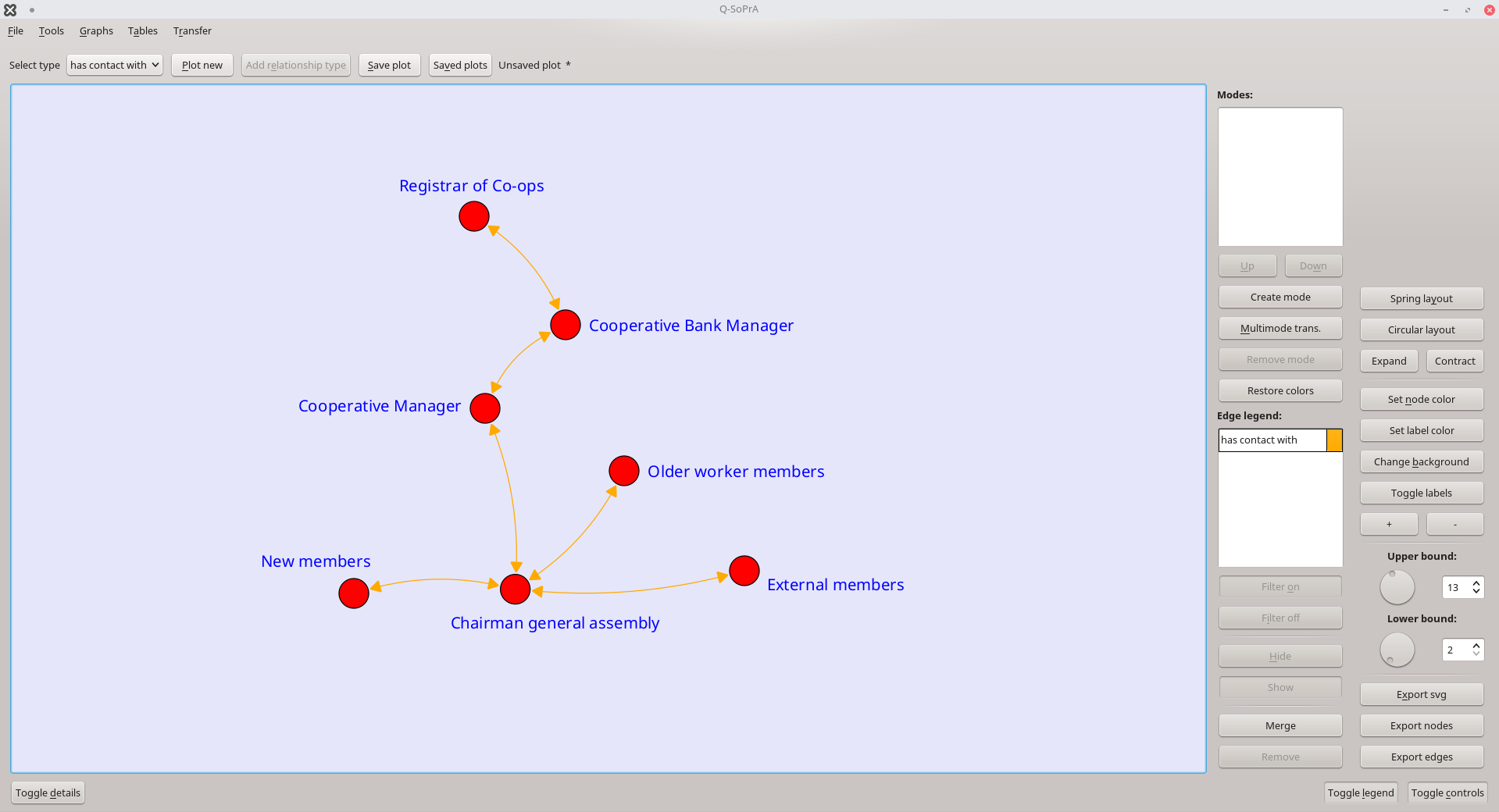
We can also change the colour of the current relationship type by double clicking its colour in the legend. This will also open the colour-picking dialog, where you can select the colour you would like to change to. In screenshot below, I have changed the colour of the nodes to red, I have changed the colour of the labels to blue, and I have changed the colour of the relationship type has contact with to orange. There is no other consequence of these changes beyond the visual ones.

Adding additional relationship types

Now let’s make things a little bit more interesting. I will add another relationship type, in this case the conceived of relationship type that we saw earlier. I can do this by selecting this relationship type from the drop-down menu in the top left of the screen, and by clicking the Add relationship type button (Clicking Plot new would just overwrite the current plot). As the colour of this relationship, I pick dark blue in this case.

Q-SoPrA will add the relationship type, as well as any new entities that this relationship type introduces to the network. The upper and lower bounds of the network filter will be reset, as well as the layout. The result can be seen in the screenshot below (I did adjust the position of the nodes and the labels already).

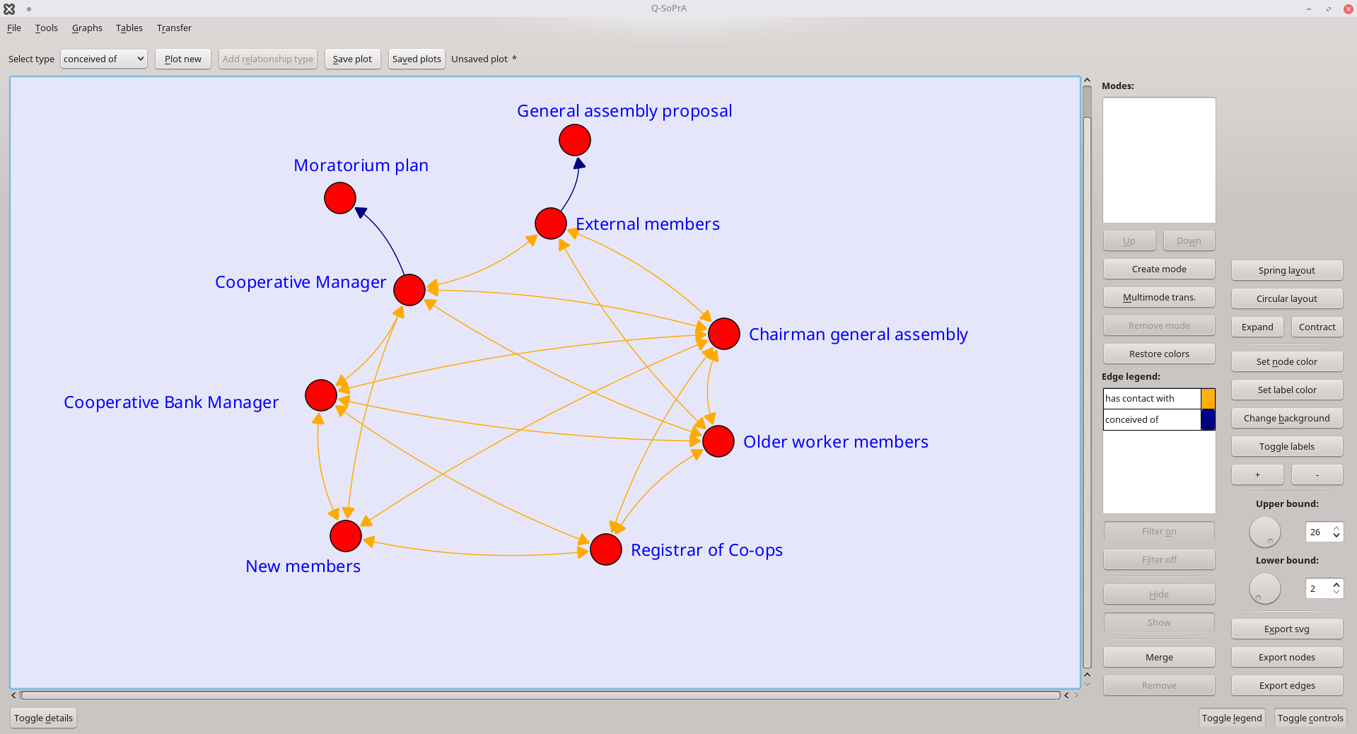
You can see that our legend now has two entries. You may also notice that two new entities have been added to the plot, namely the Moratorium plan and the General assembly proposal. If we would inspect their details, we could see that I assigned the attribute Plan to both these entities.

Creating modes

So now we have a network with two quite different types of nodes, but we haven’t made this explicit yet in the visualisation. We can do this by assigning modes to the network (see this blog post if you don’t know what modes in a network are). In Q-SoPrA, modes can be assigned to nodes based on attributes that we associated with entities. One attribute that I used while creating entities is the Actor attribute. If I want to create a new mode based on this attribute, I can click the Create mode button near the top of the Legend menu. This will open a screen with our tree of entity attributes, where we can select an attribute, as well as a node colour, and a label colour to be associated with that mode (see below).

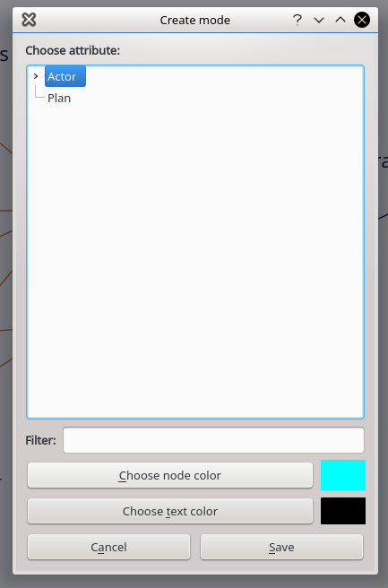
In the example above, I have selected to create a mode based on the Actor attribute, and I set the node colour to light blue, and the label colour to black. I used the same procedure to create a second mode, using the Plan attribute, but here I set the node colour to green, and the label colour to black. The results of these operations are shown in the screenshot below.

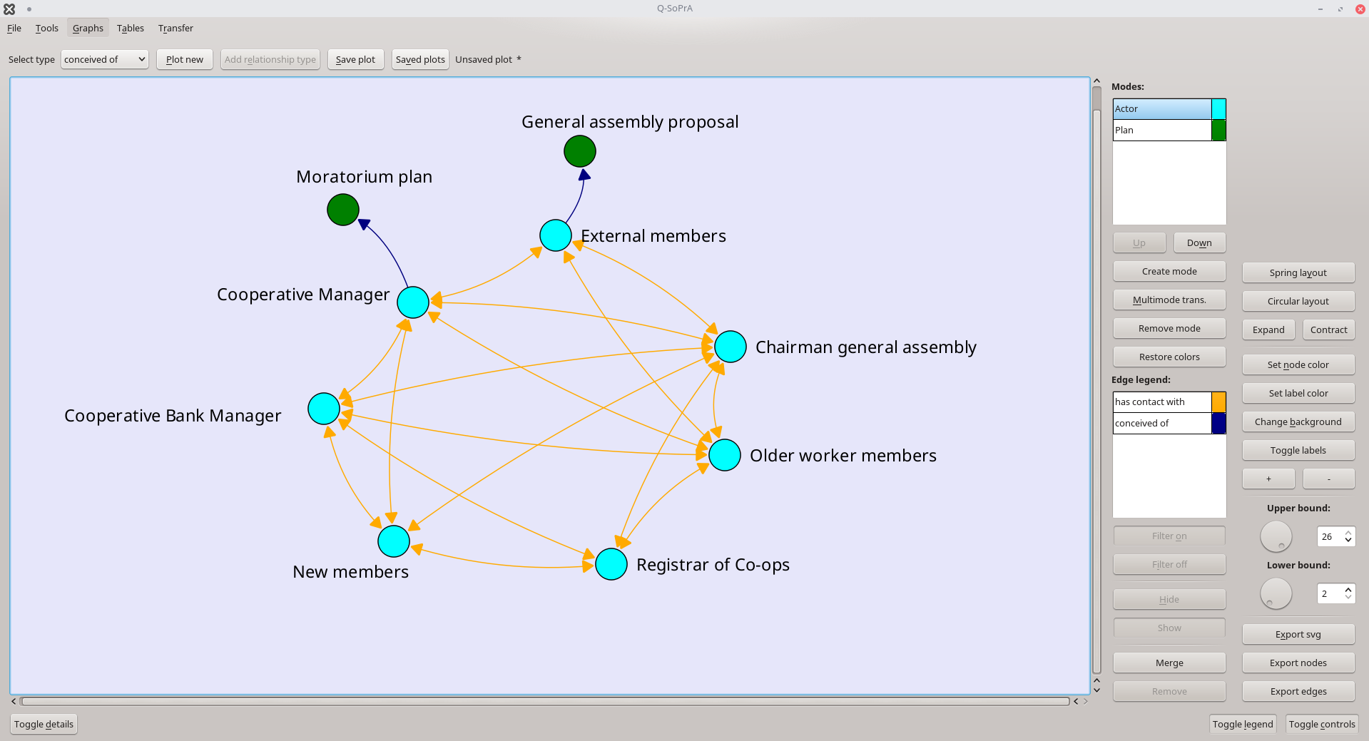
You can see that Q-SoPrA has automatically changed the colours of the nodes and the labels. Q-SoPrA does this by looking through all entities that were assigned the attribute that serves as the basis for a mode, and then classifying the matching entities in the appropriate mode. You will also see that we now have another legend, which lists the modes that we have just created (the top part of the Legend menu).

It is of course possible that an entity could be classified in multiple modes, based on the attributes assigned to it. However, any node in the network is allowed to be in only one mode at the same time. Q-SoPrA decides which mode a given entity should be assigned to based on the order in which the modes appear in the mode legend. Modes to the top of the list are always assigned first, which means that modes lower in the list may overwrite those higher in the list.

For example, if we now decide to create yet another mode, using one of the children of the Actor attribute (like Individual actor), we will see that some nodes that were previously in the Actor mode will now be in the Individual actor mode (see screenshot below).

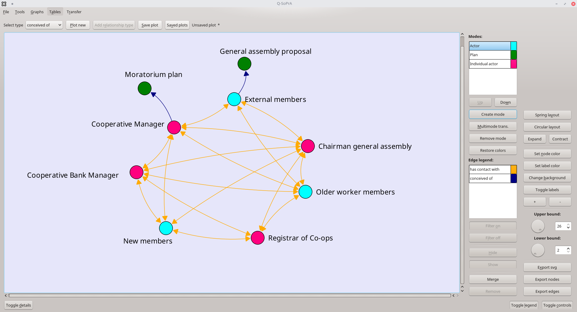
By now, we have a three-mode network, although technically we don't. Yes, that is confusing...

The reason why I say this is that in graph theory, two-mode networks are typically only considered to be two-mode networks if they are structurally bipartite. A network is bipartite if relationships only exist between nodes of two different modes, and never between nodes of the same mode.

In other words, whether or not a network is bipartite is essentially a structural question; we could determine that a network is bipartite by only looking at the patterns of relationships in the network, and without knowing anything about attributes that were assigned to the nodes.

It is of course possible that the graphs you create in Q-SoPrA are also bipartite (or maybe even tripartite) in this structural sense, but this makes no difference for how modes are interpreted in Q-SoPrA, which is purely attribute-based.

Since my last post, on attributes in Q-SoPrA, I have actually implemented a new feature, which allows you to change the order in which modes are assigned in the network graph widget and the event graph widget (discussed briefly in my last post). We can do this by selecting a mode, and then using the Up or Down buttons to change its position in the list. So, if we move the Actor mode to the bottom of the list, this means that the Individual Actor mode will be overwritten, as shown below. This allows you to control in a bit more detail how modes are assigned to nodes in the network.

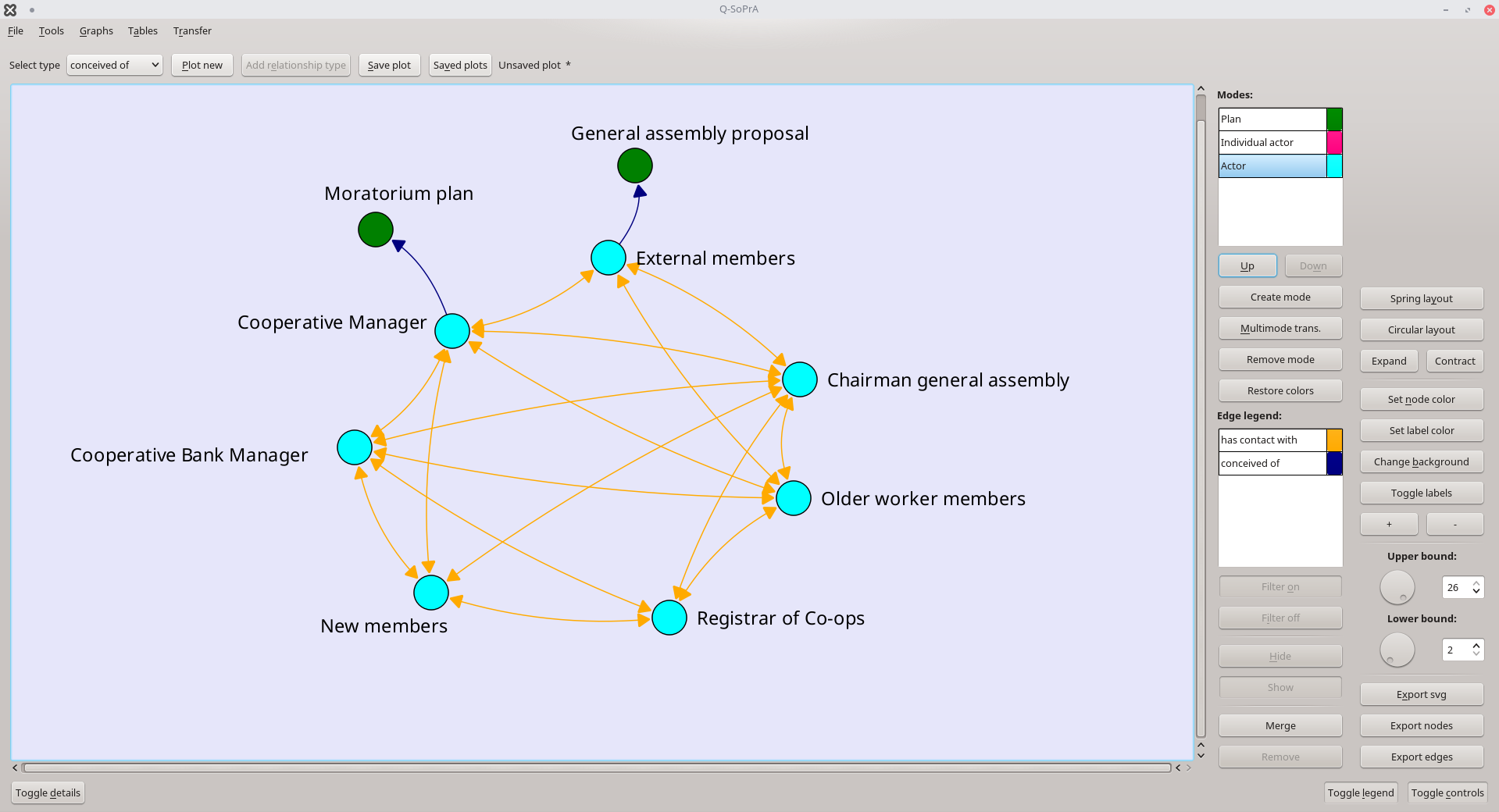
This might be a good place to also write something about mode transformations, but with our current graph, there would not be an interesting transformation to look at. Let us therefore first add a little bit more complexity to our graph.

Parallel edges

Q-SoPrA allows you to visualise parallel edges between nodes. These exist when multiple relationships exist between the same pair of nodes. To demonstrate this, I will add three additional relationship types to the graph, showing which actors have (1) shown support for certain plans, (2) offered resistance against them, or (3) shown a somewhat neutral interest in plans (that is, not being explicitly supportive, but also not dismissive of a plan).

The resulting network is show below. The graph is quite complex, since all relationships observed over the entire case study period are visualised. Some actors changed their stance towards plans over time. For example, older worker members were first resistant against the Moratorium plan, but later on started showing mild interest, before finally giving the plan full support. Indeed, to see this development, we could simply change the lower and upper bounds of the network visualisation to filter the network, but in this case I want to demonstrate how parallel edges are visualised.

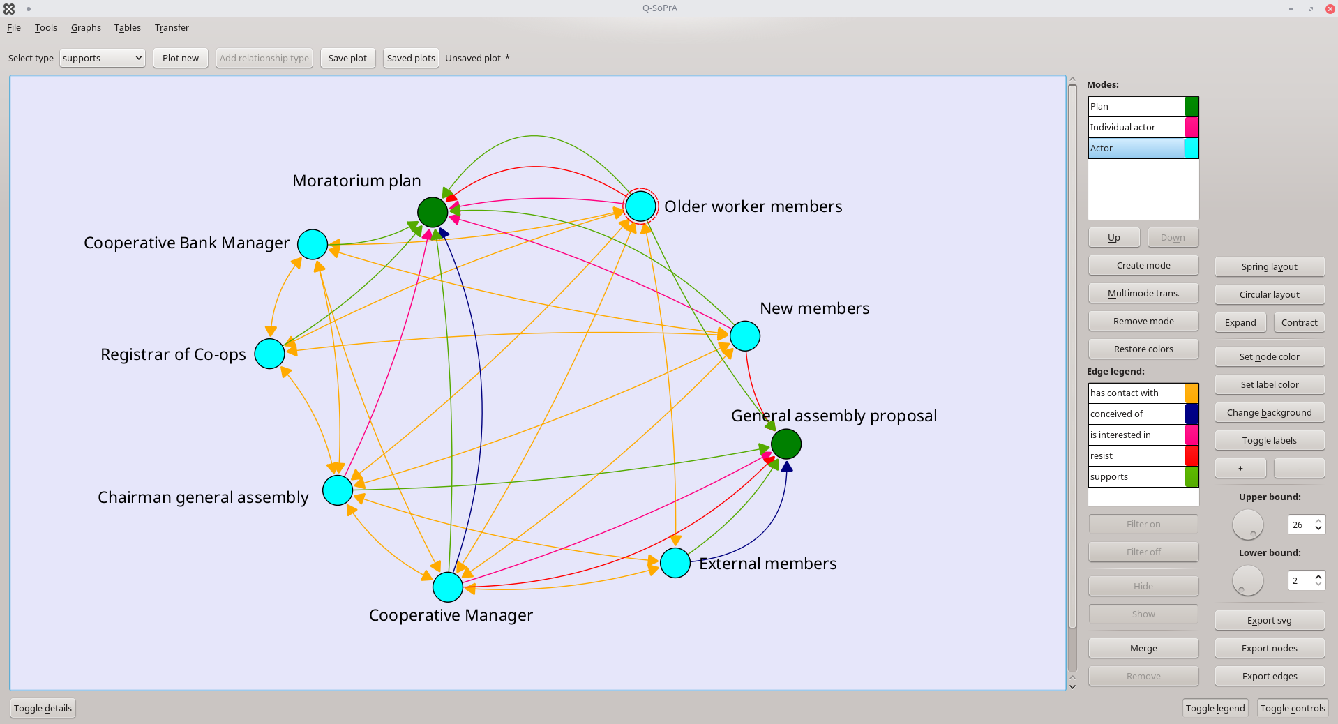
You will see that three edges are directed from the Older worker members entity to the Moratorium plan entity, capturing the three different attitudes that the former have had towards the latter. Q-SoPrA will automatically increase the ‘height’ of edge curves if another edge between the corresponding pair of nodes is already visible.

Mode transformations

Now that we have a slightly more complex network, more interesting options for performing mode transformations arise. I think of mode transformations as a way of inferring ‘latent’ (not empirically observed) relationships from empirically observed ones.

For example, imagine that we have a case study, in which we empirically observe (1) that some actors communicate with each other, and also (2) that some actors organise activities together. It is possible that we did not empirically observe some actors that co-organise activities also communicating with each other. However, it would actually make sense to assume that they did, because how will you co-organise something without getting in touch with each other?

We could of course solve this by assuming that co-organisation entails communication, and thus assigning both relationship types to an incident whenever that incident describes an instance of co-organisation of activities. However, to keep things simple, I like to stick to relationships that I can observe more or less directly in my data, and it can be quite difficult to keep the level of concentration required for this type of double-coding. Therefore, I instead choose to tell Q-SoPrA that whenever two actors co-organised something, that must mean that they have been communicating as well. This is what mode transformations can be used for.

In the example case study that we have here, we’ll look at a slightly different situation. We now have a network with several actors who have relationships to each other, but also to plans that have been conceived during the process of interest. One thing we could look at is to see if we can identify coalitions around plans based on the attitudes that actors have towards them.

One way to do this would be to say that actors are in a coalition if they support the same plans, or if one of them conceived of a plan, and the other supports it. Creating a new relationship based on these situations will involve multiple transformations.

Let us first simplify our network a bit by removing some of the relationships that we won’t be working with, that is, only keeping the conceived of and supports relationships. We can do this by selecting them in the edge legend, and then clicking the Remove button at the bottom of the Legend menu. See the result below.

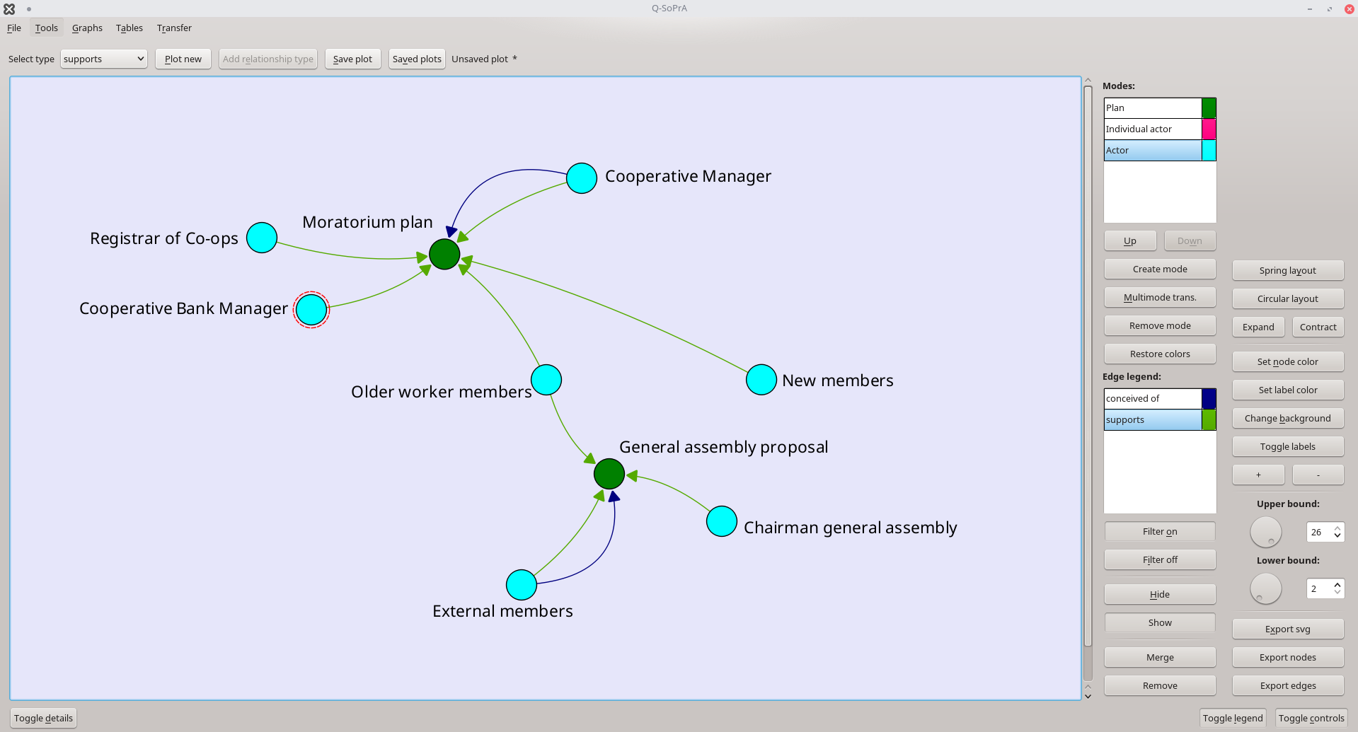
Our next step could be to create a new relationship type based on situations where one actor conceived of a plan, and another actor supports that plan. After that we will create yet another relationship type for situations where two actors support the same plan. We will later merge these relationships into one. Since it is not possible to create a new relationship type with a label that is already taken by existing one, I will take the following steps:

1. I will create the first new relationship type and call it is in coalition with A.
2. I will create the second new relationship type and call it is in coalition with B.
3. I will merge the two new relationship types in a third one and call it is in coalition with.

As you will see, merging two relationships will actually remove their original versions from the plot (but not from the data set, unless the relationships were created through transformations, as is the case in this example).

So let’s start with the first new relationship type. To create it, I click the Multimode trans. button (short for Multimode Transformation). This will open the dialog shown below (where I have already chosen my settings).

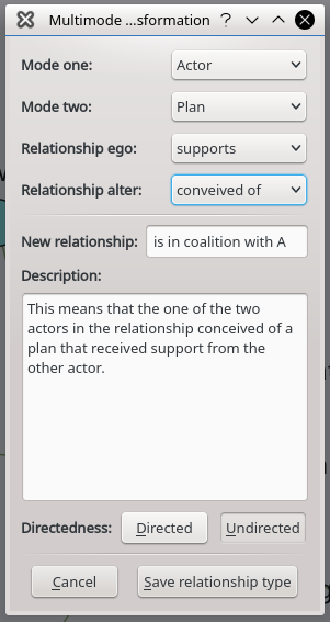
This dialog can be quite confusing when you first use it, or when you are unfamiliar with mode transformations (also, I take a somewhat different approach than is commonly used in other software, possibly adding to the confusion).

We first have to select the modes that will be part of this transformation. We want to create a new relationship type between nodes of the mode Actor, based on the relationships that these nodes have to nodes of the mode Plan. The first mode to select in this dialog (Mode one) should always be the mode among which the new relationship type can exist. So, in this case we set Mode one to Actor. The second mode should always be the mode to which nodes of the first mode might have a shared relationship (this is exactly like co-affiliation), so in this case we select Plan for Mode two.

We are not finished yet. We also have to set the relationship types that are to be considered for this transformation. It is possible that our nodes in the Actor mode have different types of relationships to nodes in the Plan mode, which is actually true in this case: Some actors conceive of plans, while others support them. In this case, we set Relationship ego to supports, and we set Relationship alter to conceived of. Why does it matter which relationship type we assign to ego or alter? Well, in this particular case it actually doesn’t matter. However, imagine that we were creating a relationship type called is supportive of, which is a directed relationship from actors that support plans to actors whose plans they are supportive of. In this case, we would thus want to create a directed relationship type from ego to alter, and then it matters which relationship types are set for ego and alter in the multimode transformation dialog.

If this is not clear, then simply trying out different settings will probably clarify things.

When we have set the relationship types, we get to the easy part: We need to create a label for the new relationship type, as well as a description. Finally, we need to choose the directedness of the relationship, which in this case we set to Undirected. Now we can save our new relationship type (we will be asked to pick a colour for the new relationship type), and it will be added to the graph. See the result below.

The multimode transformation dialog will only allow you to pick between modes and relationship types that are visible in the current network. This helps to simplify the procedure somewhat.

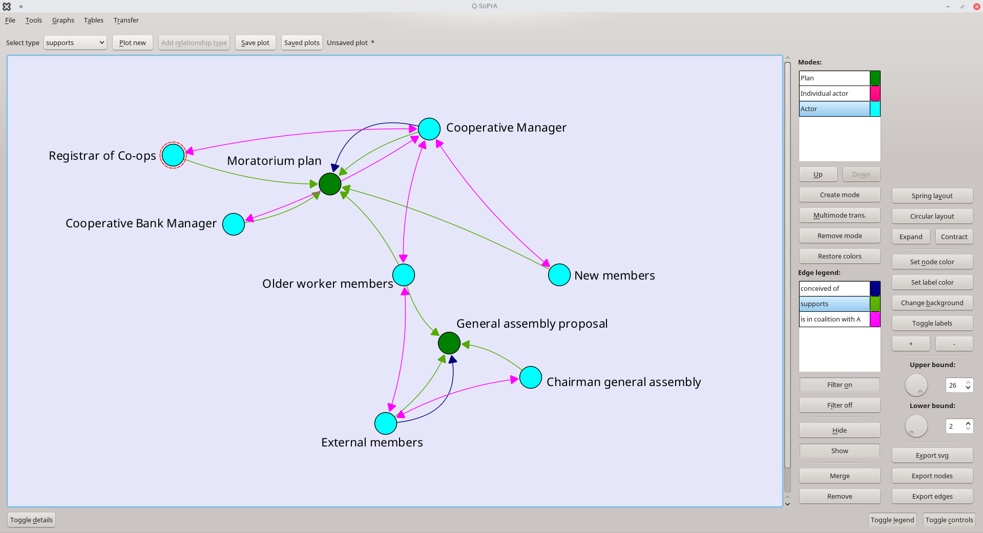
So, the first step is done. You will see that I have added a new relationship type with a pink-ish colour, and which exists between pairs of actors where one of those actors conceived of a plan, and the other actor supported that plan.

Now let’s add the other relationship type. We again open the multimode transformation dialog. We set the modes in the same way we did the last time, but now we set the relationships of both ego and alter to supports (see below).

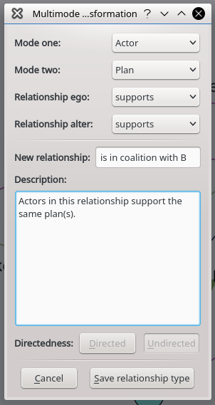
As you will see in the screenshot of the dialog above, with these settings the options for choosing the directedness of the relationship are not available. Since we have set the relationship type for both ego and alter to the same type, it would not make sense to create a directed relationship based on this transformation. Essentially, we do not even have a way to really distinguish between an ego and an alter in this case.

For our second relationship type, I have chosen the colour light blue. The result of our second transformation is shown in the screenshot below.

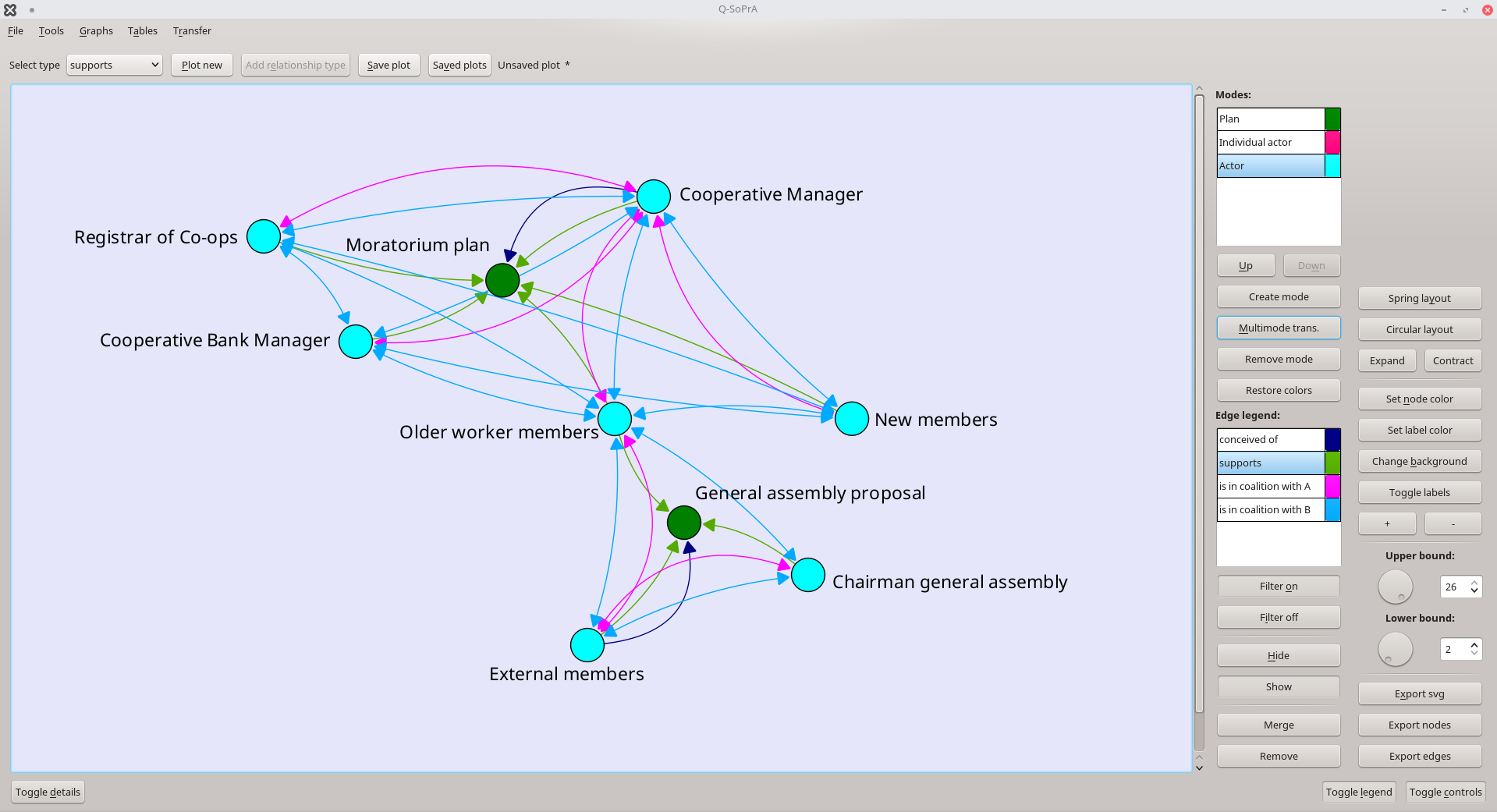
I think the graph is quite pretty like this, but it is not really easy to read. Also, our two relationship types still exist separately from each other. To merge the two relationships, we can use the Merge option near the bottom of the Legend menu. This will open the dialog shown below.

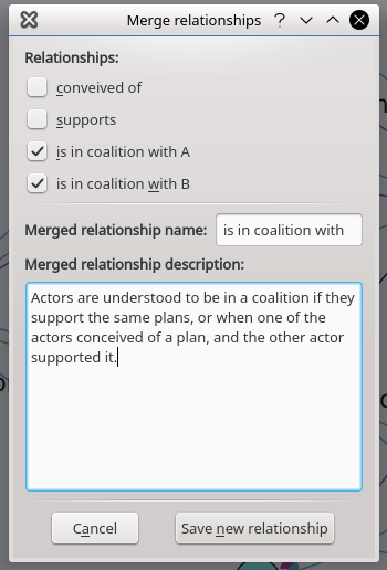
In this case we are shown a list of check boxes, where each check box represents one of the currently visible relationship types. We can use the check boxes to select the relationship types that we wish to merge (we can select more than two). It is not possible to merge relationships that have a different directedness (directed vs. undirected).

We are also asked to provide a label and a description for the new relationship type. Then, after saving the new relationship, we are again asked to pick a colour (I picked the colour black this time), and the new relationship will be added in the graph. At the same time, the relationships that we merged will be removed. See the result below.

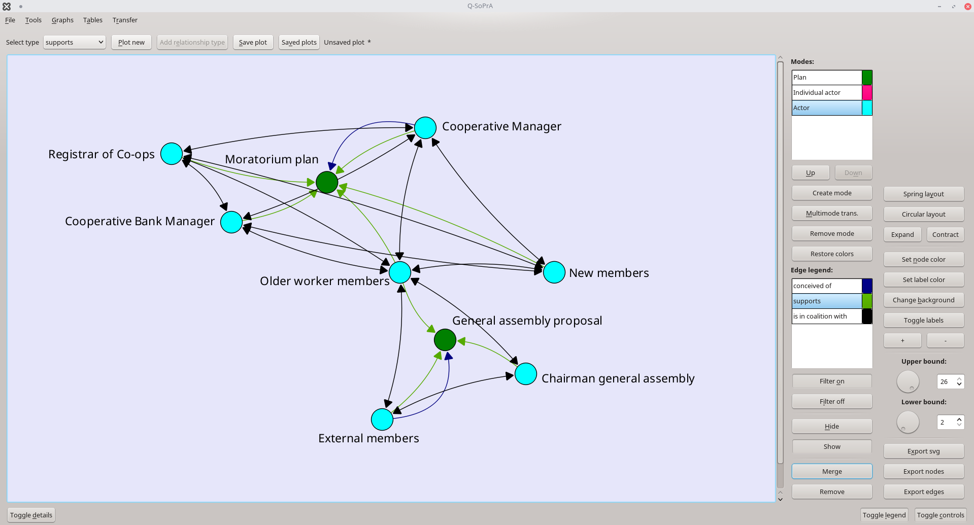
You can see that our network has already become much simpler after the merger. If we are interested in looking specifically at coalitions, we can hide the other relationship types to simplify things even further. We select them in the edge legend, and click the Hide button for each.

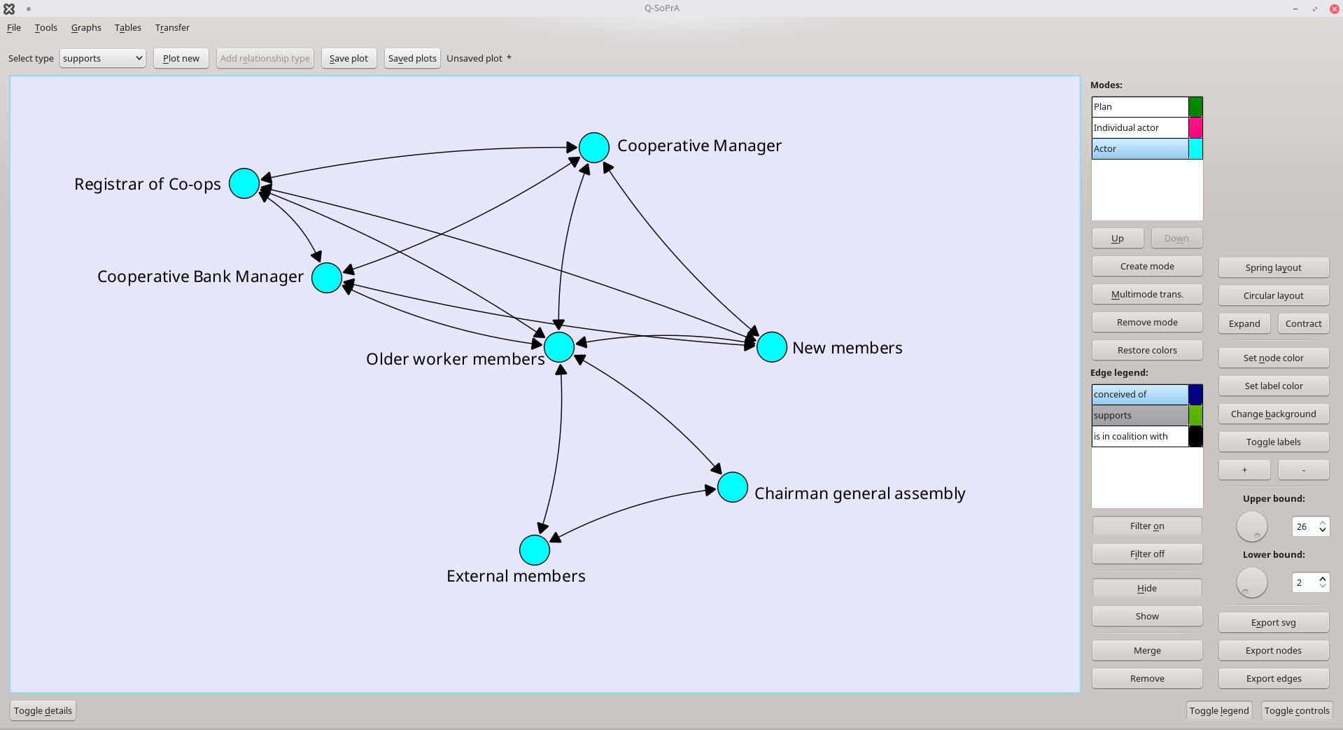
We can now see our new relationship type more clearly. We can see a coalition around the General assembly proposal in the bottom, and we can see a coalition around the Moratorium plan in the top. We can also see that there is one actor that appears in both coalitions (Older worker members).

While making these transformations, we did actually also lose some information. For example, the newly created relationship types are no longer filterable, because they are not themselves associated with any particular incidents. Thus, if you want to create such networks for a more specific episode of the process, you will have to filter the network from the very beginning. If you wish to compare the network at different points in time, you will have to repeat this procedure several times.

Exporting data

We have now already discussed quite some details about how relationships can be used in Q-SoPrA. One thing that we haven’t discussed is the possibility to calculate network metrics. I will immediately say that it is not possible to do this in Q-SoPrA… yet. I do have long-term plans to support the calculation of network metrics, but there are a couple of difficulties that are hard to overcome. For example, in Q-SoPrA you can create quite complex networks, with multiple types of relationships that may differ in directedness. It will be a challenge to create an interface for network metrics that takes all these nuances into account. I want to prevent a situation in which one calculates network metrics that actually do not make a lot of sense for the type of network structure under consideration (for example, certain network measures for one-mode networks have to be adapted before they can be applied to two-mode networks).

For now, I work with a much simpler solution: I allow the user to export network data from Q-SoPrA, which can then be imported into other software packages for further analysis. I have chosen to allow exports of node lists and edge lists that are structured in such a way that they can be imported directly into Gephi. I have two main reasons for this. First, Gephi is open source software, and I prefer to support an open source solution over a commercial one. Second, data that is imported to Gephi can be exported in many different formats. Thus, I see Gephi as a kind of gateway to other software packages. In addition, the edge list format for Gephi is quite close to the edge list formats used by some other software packages.

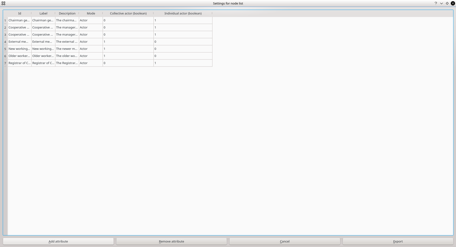
Exporting network data can be done from the Controls menu, using the Export nodes button and the Export edges button. The latter option will immediately open a dialog where you are asked to select a location and a name for your edge list, which is exported in CSV-format. If you click the Export nodes button, you will first be shown a table that shows the node list that will be exported. This list will include the Id of the nodes, the Label of the nodes (the labels are actually identical to the Ids, but this has something to do with how I typically structure the node lists I import into Gephi), the Description of the entities associated with the nodes, and the Mode that the nodes are in (this will be blank if no modes were assigned).

In this screen, you can add additional variables to the node list, by clicking the Add attribute button. Attributes can be added as a boolean, or as a valued variable. Boolean variables simply indicate whether or not a given attribute was assigned to a node. When you select to add an attribute as a boolean, than a 1 will be inserted in the new column if (a) the selected attribute was assigned, or (b) one of the children of the selected attribute was assigned. A 0 will be inserted in all other cases. If you select the option to add valued variables, then only the values assigned to the selected attribute will be considered (and not its children). Assigning values to attributes is not something I discussed in this post, but it works exactly the same as explained in my earlier post on attributes.

In the screenshot below, you see an example where I have added two attributes to the node list that indicate, respectively, whether a node has the attribute collective actor and whether a node has the attribute Individual actor. After adding attributes, the final node list can be exported as a CSV-file by clicking the Export button. This will also automatically close this dialog.

It is also possible to export the visualisation of the network graph you have created. This can be done by clicking the Export svg button in the Controls menu. This will open a dialog where you are asked to provide a name and location for the SVG-file. The SVG-file can be opened with Inkscape, which is another wonderful open source tool. In Inkscape you will be able to manipulate your graph further (each element of the graphic can still be manipulated individually), and then export it as (for example) a PNG file or a PDF, with several options to determine the resolution of the exported graphic.

Final comments.

This concludes my discussion of relationships in Q-SoPrA. I hope it has given you some ideas about how Q-SoPrA can be used for (mostly qualitative) network analysis.